Niko's Project Corner

---

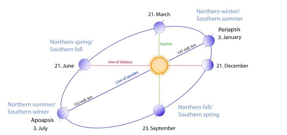
I wanted to find or cre­ate a for­mula which would ac­cept an epoch times­tamp, lat­itude and lon­gi­tude and it would pro­duce the Sun's ob­served az­imuth and al­ti­tude in ra­di­ans. It needs to take into ac­count de­tails earth's ax­ial tilt and its po­si­tion on its or­bit around the sun. To my sur­prise I wasn't able to find such for­mula, so I had to de­velop it from scratch. Luck­ily earth's or­bit (and or­bits in gen­eral) is a well stud­ied and doc­umented prob­lem, so I could take some short­cuts.

Ke­pler's equa­tion does not have an an­alyt­ical so­lu­tion, but it is easy ap­ply in the "op­po­site" di­rec­tion. Here an ap­prox­imate so­lu­tion is cre­ated. First an even sam­pling of true anoma­lies is gen­er­ated, cov­er­ing the whole 360° or­bit ro­ta­tion:

θ = 0 ... 2 π(1)

Next cor­re­spond­ing ec­cen­tric anomaly E is cal­cu­lated from θ and the or­bit's ec­cen­tric­ity e:

E = atan2(√1 - e  · sin(θ / 2), √1 + e  · cos(θ / 2))(2)

Mean anomaly M is cal­cu­lated from E by us­ing Ke­pler's equa­tion:

M = E - e sin E(3)

The M is triv­ial to cal­cu­late for any de­sired cal­en­dar date, so we want to have an ap­prox­ima­tion for­mula θ = f_e(M) so that pre­vi­ous equa­tion hold rea­son­ably well. I no­ticed ex­per­imen­tally that it would be a good ap­proach to ap­prox­imate

f'_e(M) = (M - θ) / e(4)

for e > 0, and has a some­what con­stant shape for small val­ues of e. Then the fol­low­ing holds:

θ = f_e(M) = M - e · f'_e(M)(5)

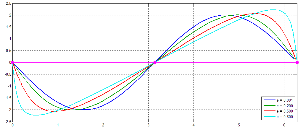
The ef­fect of e on f'_e(M) shape can be seen in Fig­ure 2. Most im­por­tantly its mag­ni­tude is around ±2, and has val­ues of ex­actly zero at M = 0, M = π and M = 2π. Due to these prop­er­ties, it is ap­prox­imated by the poly­no­mial

f'_e(M) → a(e) · (M - pi) · (M · (2π - M))^-b(e)(6)

The shape of f'_e(M) for var­ious val­ues of e can be seen in Fig­ure 2. It is no­table that for M → π / 2 it has a value of about -2, which in­di­cates that θ > M around that re­gion. This oc­curs be­cause when M → 0 the planet is clos­est to the Sun, which means it has a higher an­gu­lar ve­loc­ity. Thus θ grows ini­tially faster than the mean anomaly M.

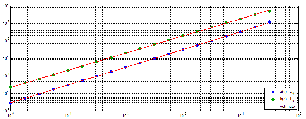
The ec­cen­tric­ity e's role on a(e) and b(e) is solved by find­ing op­ti­mal a and b for var­ious dif­fer­ent val­ues of e and fit­ting a model to those find­ings. Pa­ram­eters are es­ti­mated by min­imiz­ing the stan­dard sum of squared er­rors, which is achieved by Mat­lab's lsqnonin func­tion. These re­sults are shown in Fig­ure 3. Luck­ily both pa­ram­eters seem to fol­low the same for­mula y(e) = y₀ + exp(k₁· log(e) + k₂), and k₁ and k₂ can be reliably estimated by fitting a linear trend to the log-log data points. The constant y₀ (which corresponds to a₀ and b₀, one for both parameters) is estimated so that the best log-linear model can be obtained. If that value is off then the log-log plot is no longer linear, and a more complex model is needed.

Model ac­cu­racy is de­ter­mined by cal­cu­lat­ing the max­imum er­ror from the true lo­ca­tion within the whole 360° or­bit. If e = 0 then the or­bit would be ex­actly cir­cu­lar and θ = M. In­ter­est­ing cases are small val­ues of e, for ex­am­ple on earth's or­bit e → 0.0167. Two dif­fer­ent mod­els are com­pared in fig­ures 5 and 6: a sim­pler model which only uses con­stants a₀ and b₀ regardless of the value of e, and the more accurate model with e-dependent corrections.

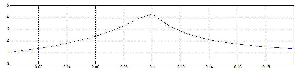
The biggest ben­efit of these cor­rec­tions oc­cur when 0.05 < e < 0.3. When e → 0 these corrections are small anyway, and on bigger values of e the model loses its accuracy even with these corrections. The ratio of simple model's maximum error and better model's error is show in Figure 4. When e = 0.1 the maximum ratio of 4 is reached, which means that the simpler model has 300% higher maximum error than the e-corrected version.

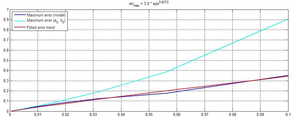
Er­ror rates (in de­grees) and the fit­ted trend curve for 0 < e < 0.1 are shown in Figure 5. Within this region the error seems to grow approximately linearly in respect to e, and for Earth's e → 0.0167 the maximum error is less than 0.1°. It should be sufficient for most applications.

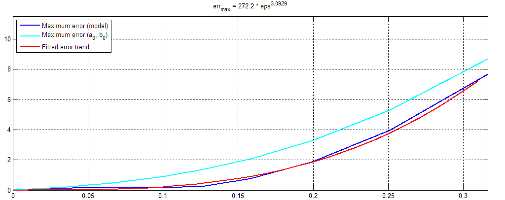
Er­ror rates for e-val­ues of up-to 10^-0.5 → 0.3 are show in Figure 6. In this context the error grows in proportion to e^3.09, reaching a maximum error of 6° at e = 0.3. It might be too high for most applications, but this elliptic orbits are not common in at least our solar system. Our top-3 planets with highest eccentricities are Mercury (e = 0.21), Mars (e = 0.09) and Saturn (e = 0.05). Pluto has a remarkably high eccentricity of 0.25.

Af­ter this model is in place, it en­ables us to cal­cu­late Earth's lo­ca­tion in re­spect to Sun in po­lar co­or­di­nates for a given times­tamp. It just needs to be con­verted to "sec­onds since Jan­uary 1 of this year", which is fur­ther con­verted to the mean anomaly M (in ra­di­ans). True anomaly θ is cal­cu­lated as

θ _e(M) = M - e · a(e) · (M - pi) · (M · (2π - M))^-b(e)
a(e) = a₀ + exp(a₁· log(e) + a₂)
b(e) = b₀ + exp(b₁· log(e) + b₂) (7)

Es­ti­mated pa­ram­eters are:

a₀ = 0.0804
a₁ = 0.9869
a₂ = 1.0123
b₀ = -1.3848
b₁ = 0.6143
b₂ = -1.0715 (8)

The next step would be to es­ti­mate the lo­cal co­or­di­nate sys­tem from lat­itude, lon­gi­tude and time, and to use po­lar co­or­di­nates to cal­cu­late the per­son's ori­en­ta­tion with re­spect to the he­lio­cen­tric co­or­di­nate sys­tem where pe­ri­ap­sis (around 3.1. each year) is the "zero" di­rec­tion. Then the Sun's ap­par­ent al­ti­tude and az­imuth can be eas­ily cal­cu­lated.

---

Related blog posts:

Bruteforcing Countdown numbers game with CUDA, 2023 Apr (Matching: Applied mathematics)
Satellite crash course, 2021 Jun (Matching: Applied mathematics)
Simulating gravitational field near a torus, 2016 Apr (Matching: Applied mathematics, Matlab)
Automatic map stitching, 2014 Sep (Matching: Matlab)
Image distortion estimation and compensation, 2014 Aug (Matching: Matlab)