Niko's Project Corner

Hu­mans are nat­urally ca­pa­ble of sep­arat­ing an ob­ject from the back­ground of an im­age, or speech from mu­sic on an au­dio clip. Photo edit­ing is an easy task, but per­son­ally I don't know how to re­move mu­sic from the back­ground. A first ap­proach would be to use band-pass fil­ters, but it wouldn't re­sult in a sat­is­fac­tory end re­sult since there is so much over­lap be­tween the fre­quen­cies. This ar­ti­cle de­scripbes a su­per­vised learn­ing ap­proach on solv­ing this prob­lem.

The used dataset con­sists of four sep­arate pod­casts (8.4 hours in to­tal) and four dif­fer­ent gen­res of mu­sic (ide­ally with­out any lyrics, 7.1 hours in to­tal). The used pod­casts were:

• Tom Se­gura & Bert Kreis­cher, 1.2 h: Ep. 105 | 2 Bears, 1 Cave w/ Tom Se­gura & Bert Kreis­cher
• Lex Frid­man, 2.4 h: Jimmy Pe­dro: Judo and the Forg­ing of Cham­pi­ons | Lex Frid­man Pod­cast #236
• Jor­dan Pe­ter­son, 2.2 h: Death, Mean­ing, and the Power of the In­vis­ible World | Clay Rout­ledge | The JBP Pod­cast S4: E54
• Joe Ro­gan, 2.6 h: Joe Ro­gan Ex­pe­ri­ence #1169 - Elon Musk

The used mu­sic gen­res and clips were:

• Clas­si­cal mu­sic, 3.5 h: The Best of Clas­si­cal Mu­sic Mozart, Beethoven, Bach, Chopin, Vi­valdi Most Fa­mous Clas­sic Pieces
• House mu­sic, 1 h: Pavel Khvaleev pres. PARAFRAME In­hale & Ex­hale Live Show @ Ra­dio In­tense / Pro­gres­sive House DJ mix
• Liq­uid Drum & Bass, 1.3 h: Liq­uid Drum and Bass Mix #127
• Pro­gres­sive rock (some lyrics), 1.3 h: Pro­gres­sive Rock Mix by Prog Rock Dock - Vol­ume 01

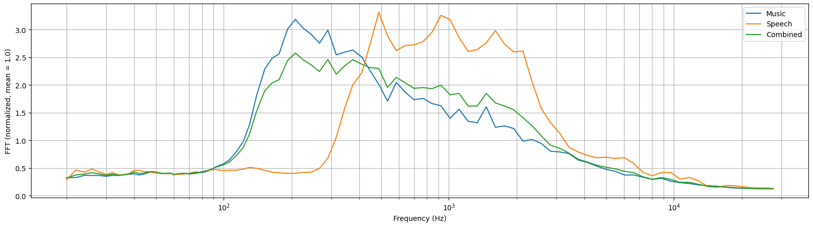
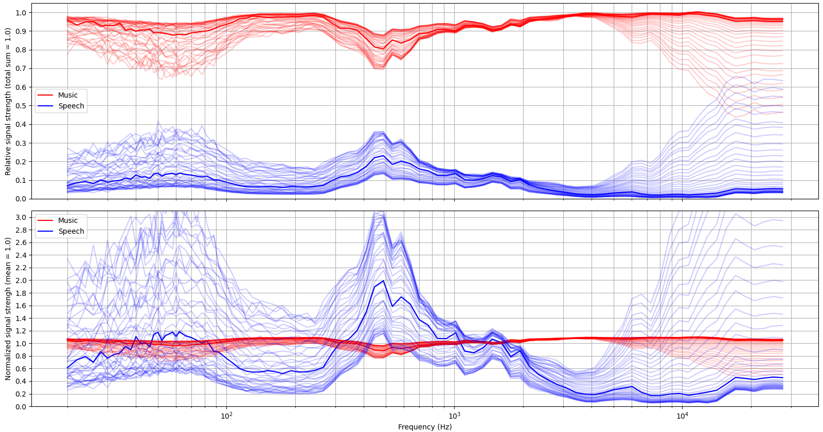
All au­dio files have a sam­pling rate of 44.1 kHz, which was down­sam­pled by 1:3 to 14.7 kHz to speed up the net­work train­ing. They were loaded to Python us­ing Py­dub, which is a wrap­per for the FFM­PEG. The files were split into two sec­ond long clips, and were nor­mal­ized so that their stan­dard de­vi­ations are one. The in­put to the net­work is a mu­sic clip + a weighted ran­dom speech clip, where the weight was picked uni­formly from the in­ter­val of [0, 1]. So there are three types of clips (mu­sic, speech and com­bined), and their av­er­aged spec­trums are shown in Fig­ure 1.

Figure 1: Spec­trums of three cat­egories of au­dio: mu­sic, speech and their com­bi­na­tion. Ob­vi­ously the "com­bined" class is found be­tween the two other classes, since Fourier trans­form is a lin­ear op­er­ation (al­though the plots are nor­mal­ized, their mean is one). The mu­sic is higher on the 100 - 400 Hz range, and speech is higher be­tween 400 and 3000 Hz.

Split­ting the 8.4 hours of pod­casts into sam­ples of two sec­onds pro­duced 15254 clips, of which 20% was used for model val­ida­tion. The in­put (1 chan­nel) and ex­pected out­put (2 chan­nels) is stored in a ma­trix of shape 15254 × 29400 × 3, which re­quires only 5.4 GB of mem­ory when stored in float32 for­mat. This fits eas­ily in RAM, but much more would be needed if more dif­fer­ent pod­casts were in­cluded, or the orig­inal sam­pling rate of 44.1 kHz was used. Nev­er­the­less there are about 360 mil­lion data points used for train­ing, and the loss is cal­cu­lated against 720 mil­lion data points.

Nat­urally sev­eral net­work ar­chi­tec­tures were ex­per­imented with, but here just the best one is de­scribed. It has three tun­able hy­per­pa­ram­eters, and they were cho­sen so that the num­ber of model pa­ram­eters was ap­prox­imately 2 mil­lion. The net­work at­tempts to nor­mal­ize the in­com­ing sig­nal's vol­ume (the vari­able stds) and re-scale the out­put back to the orig­inal level, but ex­per­iments show that for some rea­son this isn't work­ing as ex­pected.

• dim, w, n_iter = 60, 2**6, 3
• inp = Input((len_samples, 1))
• x = inp
• # Normalize the signal for the network, although this doesn't seem to work
• # as intended. Experiments show that the network isn't linear, meaning that
• # model.predict(X) * k != model.predict(X * k).
• stds = K.maximum(0.01, K.std(inp, axis=(1,2)))[:,None,None]
• x = x / stds
• x = BN()(Conv1D(dim * 2, 16*w+1, activation='elu')(x))
• x = BN()(Conv1D(dim-1, w+1, activation='elu')(x))
• # Pass the original input to refinement layers for a resnet-like architecture:
• c = (inp.shape[1] - x.shape[1]) // 2
• x = K.concatenate([x, inp[:,c:-c,:]])
• for _ in range(n_iter):
• x = BN()(Conv1D(dim, 2*w+1, activation='relu')(x) + x[:,w:-w,:])
• x = BN()(Conv1D(dim // 2, w+1, activation='elu')(x))
• x = Conv1D(1, 1, activation='linear')(x) * stds
• crop = (inp.shape[1] - x.shape[1]) // 2
• # It was evaluated that it was slightly better for the network to generate
• # the speech (2nd output) rather than the music (1st output) channel.
• model = Model(inp, K.concatenate([inp[:,crop:-crop,:] - x, x]))

On a GTX 1080TI each epoch took 13.8 min­utes, but up­grad­ing it to a RTX 3070TI (pay­ing +100% over MSRP) re­duced this by 58%, bring­ing it down to 5.8 min­utes. Any­how, the eval­uated net­work was trained with the older GPU, and full con­ver­gence took 105 epochs or 24.2 hours! Sep­arate EarlyStop­ping call­backs were used for loss and val_loss met­rics, and Adam's learn­ing rate was ad­justed down from 10^-2.5 to 10^-3.5 and 10^-4 automatically by Re­duceL­ROn­Plateau. The model was trained to a Mean Squared Error of 0.0585 for train and 0.0663 for validation.

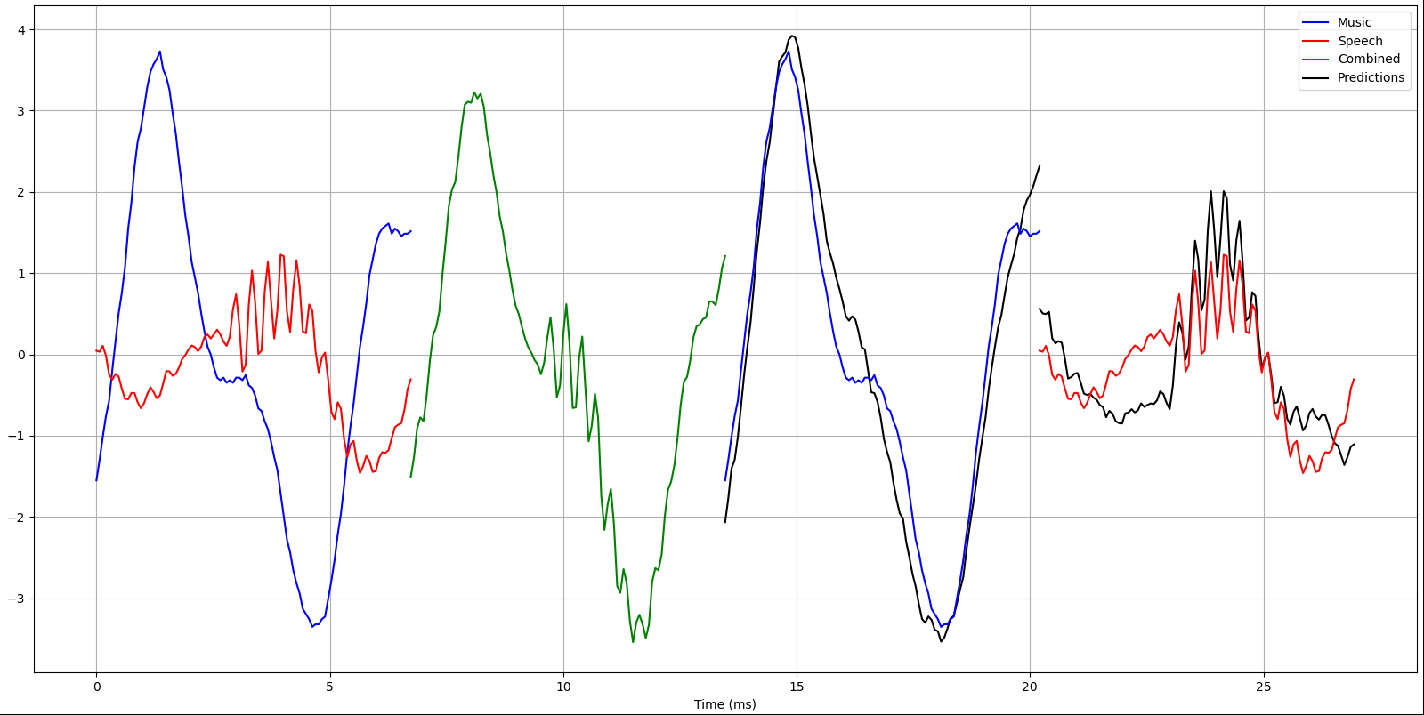
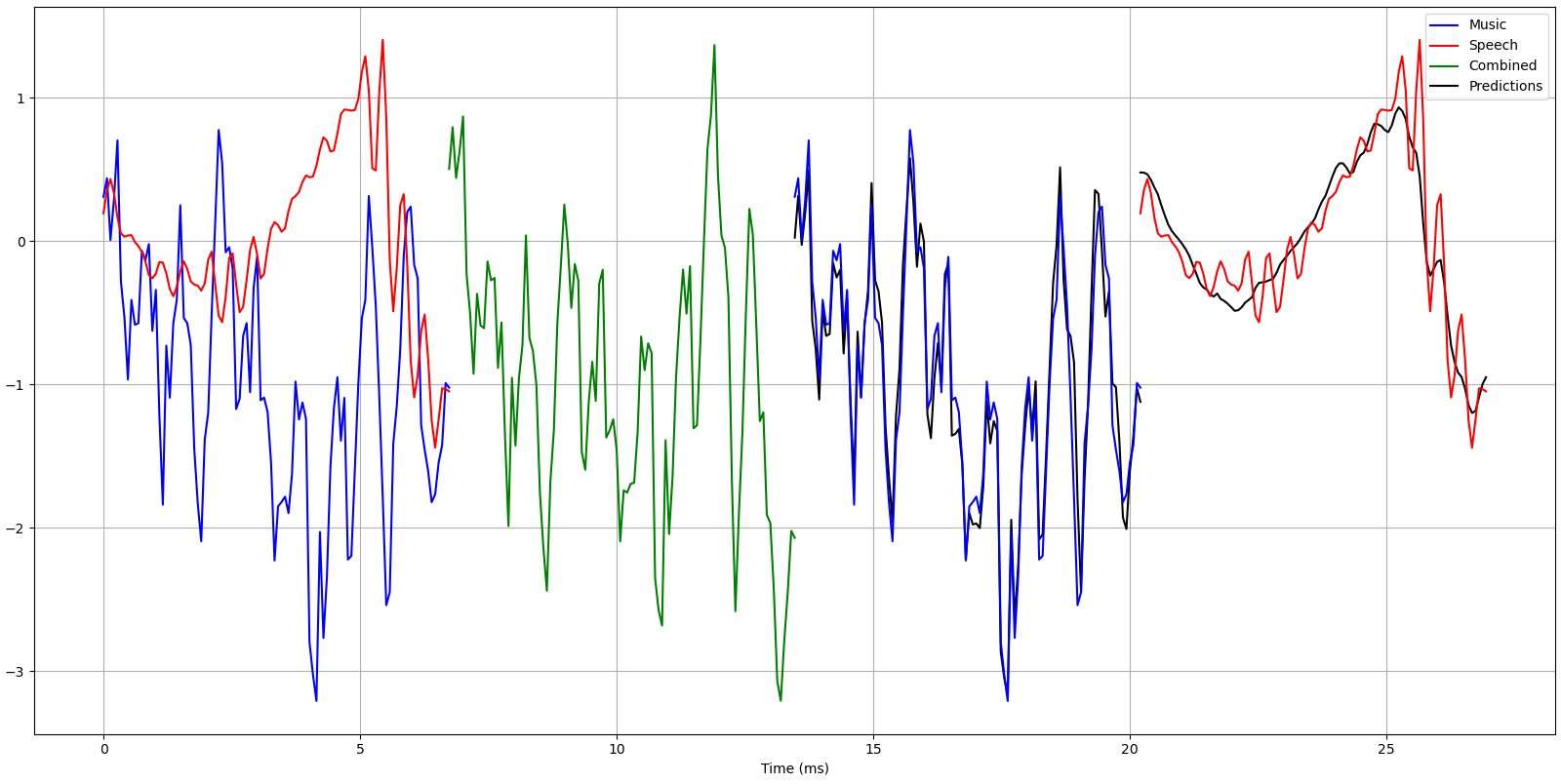
The vari­ance of the ref­er­ence mu­sic sig­nal was 1.0 as ex­pected by the nor­mal­iza­tion, but for speech it was only 0.33! Since the speech's weight is a ran­dom uni­form vari­able with a mean of 0.5, it was ex­pected that the sig­nal's mean was 0.5 as well. It was then noted that the used nor­mal­iza­tion is x /= max(1, x.std()), mean­ing that quiet sig­nals aren't go­ing to be am­pli­fied. The same for­mula was used for mu­sic, but it is plau­si­ble that a con­ver­sa­tion have quiet pe­ri­ods of a few sec­onds. Sum­ming these two un­cor­re­lated sig­nals to­gether pro­duces the in­put to the net­work, with an av­er­age vari­ance of 1.33. Com­par­ing this with the MSE loss, it is seen that the model is able to cor­rectly model about 95% of the vari­ance. Ex­am­ple in­puts and out­puts are shown in fig­ures 2 and 3.

The model's sum­mary is shown be­low:

• ___________________________________________________________________________________
• Layer (type) Output Shape Params Connected to
• ===================================================================================
• input_187 (InputLayer) [(None, 29400, 1)] 0
• tf.math.reduce_std_15 (TFOpLamb (None,) 0 input_187[0][0]
• tf.math.maximum_12 (TFOpLambda) (None,) 0 tf.math.reduce_std...
• tf.__operators__.getitem_802 (S (None, 1, 1) 0 tf.math.maximum_12...
• tf.math.truediv_10 (TFOpLambda) (None, 29400, 1) 0 input_187[0][0]
• tf.__operators__.g...
• conv1d_547 (Conv1D) (None, 28376, 120) 123120 tf.math.truediv_10...
• batch_normalization_491 (BatchN (None, 28376, 120) 480 conv1d_547[0][0]
• conv1d_548 (Conv1D) (None, 28312, 59) 460259 batch_normalizatio...
• batch_normalization_492 (BatchN (None, 28312, 59) 236 conv1d_548[0][0]
• tf.__operators__.getitem_803 (S (None, 28312, 1) 0 input_187[0][0]
• tf.concat_181 (TFOpLambda) (None, 28312, 60) 0 batch_normalizatio...
• tf.__operators__.g...
• conv1d_549 (Conv1D) (None, 28184, 60) 464460 tf.concat_181[0][0]
• tf.__operators__.getitem_804 (S (None, 28184, 60) 0 tf.concat_181[0][0]
• tf.__operators__.add_150 (TFOpL (None, 28184, 60) 0 conv1d_549[0][0]
• tf.__operators__.g...
• batch_normalization_493 (BatchN (None, 28184, 60) 240 tf.__operators__.a...
• conv1d_550 (Conv1D) (None, 28056, 60) 464460 batch_normalizatio...
• tf.__operators__.getitem_805 (S (None, 28056, 60) 0 batch_normalizatio...
• tf.__operators__.add_151 (TFOpL (None, 28056, 60) 0 conv1d_550[0][0]
• tf.__operators__.g...
• batch_normalization_494 (BatchN (None, 28056, 60) 240 tf.__operators__.a...
• conv1d_551 (Conv1D) (None, 27928, 60) 464460 batch_normalizatio...
• tf.__operators__.getitem_806 (S (None, 27928, 60) 0 batch_normalizatio...
• tf.__operators__.add_152 (TFOpL (None, 27928, 60) 0 conv1d_551[0][0]
• tf.__operators__.g...
• batch_normalization_495 (BatchN (None, 27928, 60) 240 tf.__operators__.a...
• conv1d_552 (Conv1D) (None, 27864, 30) 117030 batch_normalizatio...
• batch_normalization_496 (BatchN (None, 27864, 30) 120 conv1d_552[0][0]
• conv1d_553 (Conv1D) (None, 27864, 1) 31 batch_normalizatio...
• tf.__operators__.getitem_807 (S (None, 27864, 1) 0 input_187[0][0]
• tf.math.multiply_22 (TFOpLambda (None, 27864, 1) 0 conv1d_553[0][0]
• tf.__operators__.g...
• tf.math.subtract_91 (TFOpLambda (None, 27864, 1) 0 tf.__operators__.g...
• tf.math.multiply_22[
• tf.concat_182 (TFOpLambda) (None, 27864, 2) 0 tf.math.subtract_91[
• tf.math.multiply_22[
• ===================================================================================
• Total params: 2,095,376
• Trainable params: 2,094,598
• Non-trainable params: 778

The used er­ror ma­tric was just the plain MSE, which doesn't cor­re­sponds well on how the gen­er­ated sig­nal sounds to a hu­man ear. A bet­ter stan­dard would be the Per­cep­tual Eval­ua­tion of Au­dio Qual­ity or ... Speech Qual­ity. The lat­ter is im­ple­mented in a Python li­brary python-pesq, which could be used for model eval­ua­tion. But since it isn't dif­fer­en­tiable, it can­not be used as the model's loss func­tion.

There is also a Deep Per­cep­tual Au­dio Met­ric (DPAM) (Arxiv) metric, which is actually differentiable! However it wasn't tested, mainly because it doesn't support Tensorflow 2.x and it requires a different sampling rate (22050 Hz, all experiments were done with 44100 / 3 = 14700 Hz).

Yet an other ap­proach would be to train a net­work to cal­cu­late the sig­nal's spec­togram, and then use it as a loss (with frozen weights) in sig­nal re­con­struc­tion. I have no idea whether it would work as a stand-alone loss, or it should be used alongside with MSE. In­tu­ition tells me that if the spec­tro­gram matches, then it should sound good re­gard­less of phase shift etc.

Figure 2: Ex­am­ples of orig­inal au­dio (mu­sic in blue and speech in red), their com­bined sig­nal (green) and cor­re­spond­ing pre­dic­tions (black). Each shown sig­nal is only 100 sam­ples long, so at the sam­pling rate of 14700 Hz it rep­re­sents only about 7 mil­lisec­onds of au­dio. Note that the net­work uses a "con­text" of 768 sam­ples be­fore and af­ter each pre­dicted sam­ple. It is very hard to vi­su­ally es­ti­mate the qual­ity of the pro­duced sig­nal, since it is rep­re­sented in a time and not in fre­quency do­main. The model gen­er­ates prop­erly smooth "mu­sic" sig­nal, and the high fre­quen­cies are al­lo­cated to the "speech" out­put. And there seems to be a low-fre­quency off­set, so the black pre­dic­tion of "speech" has a rather large MSE af­ter­all.

Figure 3: An other ex­am­ple of in­put and out­puts, this time the speech out­put is miss­ing some higher fre­quen­cies and is thus too smooth. Those fre­quen­cies are leaked to the mu­sic pre­dic­tion, but they are vi­su­ally very hard to judge.

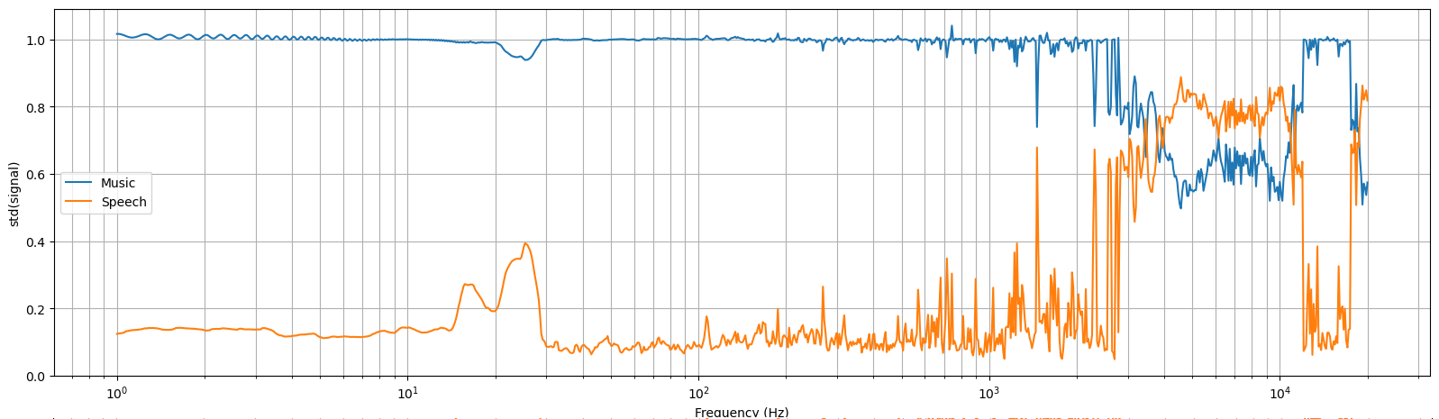
White noise (also known as Gaus­sian noise) con­tains an equal amount of all of the fre­quen­cies, and is thus of­ten used as a "test in­put" to a sig­nal pro­cess­ing unit or an al­go­rithm. Fig­ure 4 shows that what per­cent­age of each fre­quency range gets passed to the "mu­sic" or "speech" out­put. The net­work isn't con­strained to pre­serve the to­tal en­ergy, so the sum of the two out­puts may have a higher vari­ance than the in­put sig­nal. Ac­cord­ing to Ac­cu­sonus.com, hu­man speech spans from a range of 125 Hz to 8000 Hz. Ear­lier on Fig­ure 1 it was seen that this dataset's speech is dis­tinct from mu­sic at around fre­quen­cies be­tween 300 and 3000 Hz. But it should be noted that this dataset doesn't have any woman or child speak­ers. Those would be re­ally good test cases for ad­di­tional model val­ida­tion.

The net­work's re­sponse to white noise of vary­ing am­pli­tudes is shown in Fig­ure 4. 80 - 99% of the sig­nal is passed to the "mu­sic" out­put and the rest to the "speech" out­put. As ex­pected, the speech out­put is strongest at fre­quen­cies be­tween 300 and 1000 Hz. The net­work was in­tended to be co­vari­ant (or lin­ear) in re­spect to the in­put sig­nal's vol­ume, mean­ing that ide­ally pre­dict(x) · k = pre­dict(x · k). The fig­ure shows that this is not the case. At the mo­ment the rea­son for this be­hav­ior is un­known.

Figure 4: Fre­quency re­sponse of the "mu­sic" and "speech" out­puts to white noise with vary­ing stan­dard de­vi­ations (be­tween 0.6 and 1.6). A scale-in­vari­ant (ac­tu­ally co­vari­ant!) net­work wouldn't show this kind of spread on this nor­mal­ized vi­su­al­iza­tion.

In ad­di­tion to white noise, the net­work's sig­nal pass­ing was also stud­ied us­ing pure si­nu­soidal sig­nals. The re­sult is shown in Fig­ure 5, and it shows some sur­pris­ing re­sults. Al­though fre­quen­cies be­tween 300 and 3000 Hz are most dis­tinct for speech, they don't get passed to the "speech" out­put as a stand-alone sig­nal. It seems that the net­work has learned some pat­terns in speech, and it only lets those pass through. It is also un­clear why the net­work be­haves so oddly at high fre­quen­cies, maybe be­cause they aren't much pre­sent in the train­ing data.

Figure 5: Fre­quency re­sponse of the net­work to pure sin func­tions. In­ter­est­ingly the speech out­put doesn't let the pure fre­quen­cies of 300 - 2000 Hz through, even though it is the dis­tinc­tive range for speech. An other odd­ity is that it lets higher fre­quen­cies of 3000 - 10000 Hz through, but this wasn't ob­served with white noise.

Figure 6: The his­togram of cor­re­la­tion co­ef­fi­cient be­tween re­verse(pre­dict(x)) and pre­dict(re­verse(x)) shows that the model isn't time-re­versible, es­pe­cially on the "speech" cat­egory. This means that re­vers­ing the in­put re­sults in a dif­fer­ent out­come than re­vers­ing the out­put. This is anal­ogous to a CNN clas­si­fier not be­ing in­vari­ant to the im­age be­ing flipped hor­izon­tally. Maybe mu­sic is much more pe­ri­odic, and the model is quite re­versible for those sig­nals.

The in­put has 29400 sam­ples, but the out­put has only 27864 (768 · 2 = 1536 fewer). This hap­pens be­cause the net­work uses Conv1D lay­ers with­out padding, so at each layer the out­put gets a lit­tle smaller. Be­cause of this, ex­tra care has to be taken when pro­cess­ing longer in­put se­quences. The first in­put is sam­ples from 0 to 29399 (in­clu­sive), but the sec­ond in­put is not from 29400 to 58799! In­stead the "crop fac­tor" has to be taken into ac­count, so the sec­ond range is shifted left by 768. This gives us 29400 - 768 to 2 · 29400 - 768 - 1, or 28632 to 58031. The third range is from 2 · 29400 - 768 to 3 · 29400 - 2 · 768 - 1. Also the model doesn't give pre­dic­tions to the first 768 sam­ples, so the pre­dicted out­put has to be padded with that many ze­ros (ac­tu­ally I for­got to do the padding, so au­dio tracks are a bit out of sync).

Ex­am­ples of "orig­inal", "mu­sic" and "speech" ver­sions can be heard from an un­listed youtube video. Ap­plied au­dio pro­cess­ing of each clip is shown in the top left cor­ner. It has short clips from videos Eric gets over­con­fi­dent against Hikaru, DON'T WASTE YOUR TIME - Best Mo­ti­va­tional Speech Video (Fea­tur­ing Eric Thomas) and jack­ass forever | Of­fi­cial Trailer (2022 Movie). Obviously these videos haven't been used for training the model, so puts the network into a true test. Sadly the output isn't good audio quality, most notably the "music" track has very audible speech and the "speech" has noticeably lower quality than the original. At least the "speech" doesn't have much audible music.

A bet­ter re­sult might be ob­tained by us­ing more a di­verse set of train­ing data, us­ing a more com­plex model (but over­fit­ting has to be midi­gated some­how), and hav­ing a bet­ter loss func­tion than the plain MSE. Some ideas were al­raedy men­tioned ear­lier, but hav­ing the Short-time Fourier trans­form as a pre­dic­tion tar­get sounds in­ter­est­ing. Fun­da­men­tally the hu­man ear doesn't care about the phase of the sig­nal, only the com­po­si­tion of fre­quen­cies mat­ter. But the spec­trum cal­cu­la­tion has to be dif­fer­en­tiable so that Keras is able to prop­agate loss derivates through it.

Related blog posts:

Cheating at Bananagrams with real-time AI, part 1, 2023 Apr (Matching: Keras, Python)
Matching puzzle pieces together, 2022 Jul (Matching: Keras, Python)
Image and video clustering with an autoencoder, 2022 Jan (Matching: Keras, Python)
Helsinki Deblur Challenge 2021, 2021 Dec (Matching: Keras, Python)
Chess video search engine, 2021 Jun (Matching: Keras, Python)