Niko's Project Corner

---

Youtu­ber An­other Roof posed an in­ter­est­ing ques­tion on his video "The Sur­pris­ing Maths of Britain's Old­est* Game Show". The chal­lenge was stated in the video's de­scrip­tion: "I want to see a list of the per­cent­age of solv­able games for ALL op­tions of large num­bers. Like I did for the 15 op­tions of the form {n, n+25, n+50, n+75}, but for all of them. The op­tions for large num­bers should be four dis­tinct num­bers in the range from 11 to 100. As I said there are 2555190 such op­tions so this will re­quire a clever bit of code, but I think it’s pos­si­ble!". His ref­er­ence Python im­ple­men­ta­tion would have taken 1055 days (25000 hours) of CPU time (when all four large num­bers are used in the game), but with CUDA and a RTX 4080 card it could be solved in just 0.8 hours, or 31000x faster!

Al­though, there is some con­fu­sion since he says that his code took 90 min­utes to run per cho­sen four dig­its, but on my ex­per­iments with i7-6700K CPU and with­out any mul­ti­pro­cess­ing I mea­sured it to take about 0.65 sec­onds per a "game" (a set of six num­bers). When whe choose the re­main­ing two small num­bers, there are 55 dis­tinct games, so it takes just 0.65 × 55 = 35.6 sec­onds to solve for given four large dig­its. Mul­ti­ply­ing this by 2.56 mil­lion brings us to 1055 days, or 2.9 years. I guess he took into con­sid­er­ation also the games with one, two or three large num­bers se­lected out of the four. These have 5808, 3690 and 840 op­tions for the re­main­ing five, four or three small num­bers. Tak­ing also these into ac­count, it brings the to­tal es­ti­mated run­time to 546 years, which is close to his es­ti­mate of 438 years. But these vari­ants con­tain lots of du­pli­cate games, and fil­ter­ing those out drops the num­ber of games from 26606 mil­lion to "just" 208 mil­lion, or a 128x re­duc­tion! Then the whole cal­cu­la­tion would take "only" 4.3 years.

The first step is to pre-cal­cu­late all the ways of com­bin­ing the six given num­bers into new ones with bi­nary op­er­ations. This way they can be all checked in par­al­lel. That "per­mu­ta­tion" table was gen­er­ated with the fol­low­ing Python code (which has syn­tax high­lights in the PDF ver­sion):

• def gen_perms(ix_to, used):
• if ix_to == 11:
• yield []
• return
• unused = sorted(set(range(ix_to)) - used)
• for i in unused:
• for j in unused:
• # The first six numbers must be sorted in descending order!
• if i == j or (i < 6 and j < 6 and i > j):
• continue
• for p in gen_perms(ix_to + 1, used | {i, j}):
• yield [[i, j, ix_to]] + p
• perms = np.array(list(gen_perms(6, set())), dtype=np.int32)
• # perms.shape == (23040, 5, 3)

The perms vari­able has three in­te­ger in­dices per a cal­cu­la­tion "step". Since there are six num­bers, there are at most five steps in the cal­cu­la­tion. On a given per­mu­ta­tion, it lists that from which in­dices the op­er­ation's val­ues are taken, and to which slot the re­sult is writ­ten. Ac­tu­ally re­sults are al­ways writ­ten to the first free slot, so those in­dices are al­ways 6, 7, 8, 9 and 10. Ex­am­ple per­mu­ta­tions are shown be­low.

• array([[[ 0, 1, 6], [ 2, 3, 7], [ 4, 5, 8], [ 6, 7, 9], [ 8, 9, 10]],
• [[ 0, 1, 6], [ 2, 3, 7], [ 4, 5, 8], [ 6, 7, 9], [ 9, 8, 10]],
• [[ 0, 1, 6], [ 2, 3, 7], [ 4, 5, 8], [ 6, 8, 9], [ 7, 9, 10]],
• ...,
• [[ 4, 5, 6], [ 6, 3, 7], [ 7, 2, 8], [ 8, 0, 9], [ 9, 1, 10]],
• [[ 4, 5, 6], [ 6, 3, 7], [ 7, 2, 8], [ 8, 1, 9], [ 0, 9, 10]],
• [[ 4, 5, 6], [ 6, 3, 7], [ 7, 2, 8], [ 8, 1, 9], [ 9, 0, 10]]],
• dtype=int32)

It turns out that only 44.5% of these per­mu­ta­tions de­scribe an unique way of com­bin­ing the in­put num­bers. These can be eas­ily fil­tered out by check­ing what is the de­pen­dency chain of the fi­nal cal­cu­lated num­ber, which is al­ways stored to the in­dex 10. This still leaves du­pli­cate cal­cu­la­tions for com­mu­ta­tive op­er­ations of ad­di­tion and mul­ti­pli­ca­tion, but they are fil­tered out ad-hoc later in the al­go­rithm.

• is_unique = np.ones(perms.shape[0]).astype(bool)
• seen_deps = { }
• for ix in range(perms.shape[0]):
• perm = perms[ix]
• deps = { }
• for i in range(5):
• deps[perm[i,2]] = (deps.get(perm[i,0]) or (perm[i,0],)), \
• (deps.get(perm[i,1]) or (perm[i,1],))
• if deps[10] in seen_deps:
• is_unique[ix] = False
• seen_deps[deps[10]].append(perm)
• else:
• seen_deps[deps[10]] = [perm]
• perms = perms[is_unique]
• # perms.shape == (10260, 5, 3)

Here is an ex­am­ple of a cal­cu­lated de­pen­dency chain:

• array([[ 4, 5, 6],
• [ 6, 3, 7],
• [ 7, 2, 8],
• [ 8, 1, 9],
• [ 9, 0, 10]], dtype=int32)
• # ->
• {6: ((4,), (5,)),
• 7: (((4,), (5,)), (3,)),
• 8: ((((4,), (5,)), (3,)), (2,)),
• 9: (((((4,), (5,)), (3,)), (2,)), (1,)),
• 10: ((((((4,), (5,)), (3,)), (2,)), (1,)), (0,))}

Some de­pen­dency-chains are du­pli­cated up-to eight times. This is one such case:

• array([[[ 0, 1, 6], [ 2, 3, 7], [ 4, 5, 8], [ 6, 7, 9], [ 8, 9, 10]],
• [[ 0, 1, 6], [ 2, 3, 7], [ 6, 7, 8], [ 4, 5, 9], [ 9, 8, 10]],
• [[ 0, 1, 6], [ 4, 5, 7], [ 2, 3, 8], [ 6, 8, 9], [ 7, 9, 10]],
• [[ 2, 3, 6], [ 0, 1, 7], [ 4, 5, 8], [ 7, 6, 9], [ 8, 9, 10]],
• [[ 2, 3, 6], [ 0, 1, 7], [ 7, 6, 8], [ 4, 5, 9], [ 9, 8, 10]],
• [[ 2, 3, 6], [ 4, 5, 7], [ 0, 1, 8], [ 8, 6, 9], [ 7, 9, 10]],
• [[ 4, 5, 6], [ 0, 1, 7], [ 2, 3, 8], [ 7, 8, 9], [ 6, 9, 10]],
• [[ 4, 5, 6], [ 2, 3, 7], [ 0, 1, 8], [ 8, 7, 9], [ 6, 9, 10]]],
• dtype=int32)

The next step is to im­ple­ment the CUDA ker­nels. Their code is fairly ba­sic and sim­ple, and we didn't need to re­sort to more ex­oc­tic con­structs such as atomic op­er­ations, streams or warp-based vot­ing. But shared and lo­cal memory is used. The apply_op_gpu applies one calculation step (if it is valid), and stores it to the passed perm array. It discards invalid cases, which are negative numbers, too large numbers and a division which would result in a fraction.

• # Setting registers=40 to get 100
• @cuda.jit((numba.int32[:,:], numba.int32, numba.int32, numba.int32[:]),
• device=True, max_registers=40)
• def apply_op_gpu(perm, i, op, state):
• j = perm[i,0]
• k = perm[i,1]
• a = state[j]
• b = state[k]
• val = 0
• if op == 0:
• if j < k: # An optimization for commutative ops
• val = a + b
• elif op == 1:
• val = a - b
• elif op == 2:
• if j < k: # An optimization for commutative ops
• val = a * b
• if val > 0xFFFFFF:
• val = 0
• elif b > 0 and a >= b: # op == 3
• div = a // b
• if div * b == a:
• val = div
• if i < 4: # We don't need to persist the result for the last operation.
• state[perm[i,2]] = val
• return val

The pos­si­ble_tar­gets_gpu is ba­si­cally just a nested for-loop, test­ing each of the pos­si­ble 4⁵ = 1024 operation sequences. In CUDA programming threads are arranged into 3D grids, and here the x-axis loops over games (a set of six numbers), and y-axis loops over permutations. The used grid has threadblock dimensions of 1 × 128 × 1, which is a nice small multiple of 32, which the number of active threads in a warp. We don't need to do any out-of-bounds checking with x, since it is trivially matched to the first dimension of the games array. The z-axis isn't used for anything.

• @cuda.jit((numba.int32[:,:], numba.int32[:,:,:], numba.int32[:,:]),
• max_registers=40)
• def possible_targets_gpu(games, perms, out):
• # Reachable target numbers are buffered here, before writing them
• # out to the global memory. Note that 100 is missing from here, even
• # if it is a given digit. That edge-case is handled later in the code,
• # which calls this kernel and aggregates the results.
• # Also numbers 0 - 99 and 1000 - 1023 are recorded as reachable, when possible.
• # These are discarded later, to keep this code a bit simpler.
• results = cuda.shared.array(1024, numba.int32)
• for block_idx_y in range(0, (1024 + cuda.blockDim.y - 1) // cuda.blockDim.y):
• i = block_idx_y * cuda.blockDim.y + cuda.threadIdx.y
• if i < 1024:
• results[i] = 0
• cuda.syncthreads()
• x = cuda.blockDim.x * cuda.blockIdx.x + cuda.threadIdx.x
• y = cuda.blockDim.y * cuda.blockIdx.y + cuda.threadIdx.y
• # This has the six input numbers + the FOUR calculated ones (the last one
• # is ommitted, apply_op_gpu's return value is directly used from `val`).
• state = cuda.local.array(10, numba.int32)
• for i in range(6):
• state[i] = games[x,i]
• # This holds a single permutation, as determined by `y`.
• perm = cuda.local.array((5,3), numba.int32)
• if y < perms.shape[2]:
• for i in range(5):
• for j in range(3):
• # Note that `perms` has been transposed before it was copied
• # to the device, for better read-performance.
• perm[i,j] = perms[i,j,y]
• for op0 in range(4):
• val = apply_op_gpu(perm, 0, op0, state)
• if val <= 0: continue
• if val < 1024: results[val] = 1
• for op1 in range(4):
• val = apply_op_gpu(perm, 1, op1, state)
• if val <= 0: continue
• if val < 1024: results[val] = 1
• for op2 in range(4):
• val = apply_op_gpu(perm, 2, op2, state)
• if val <= 0: continue
• if val < 1024: results[val] = 1
• for op3 in range(4):
• val = apply_op_gpu(perm, 3, op3, state)
• if val <= 0: continue
• if val < 1024: results[val] = 1
• for op4 in range(4):
• val = apply_op_gpu(perm, 4, op4, state)
• if val <= 0: continue
• if val < 1024: results[val] = 1
• # Wait for all threads to have finished, and persist the aggregated
• # results into global memory.
• cuda.syncthreads()
• for block_idx_y in range(0, (1024 + cuda.blockDim.y - 1) // cuda.blockDim.y):
• i = block_idx_y * cuda.blockDim.y + cuda.threadIdx.y
• if i < 1024 and results[i] > 0:
• out[x,i] = 1

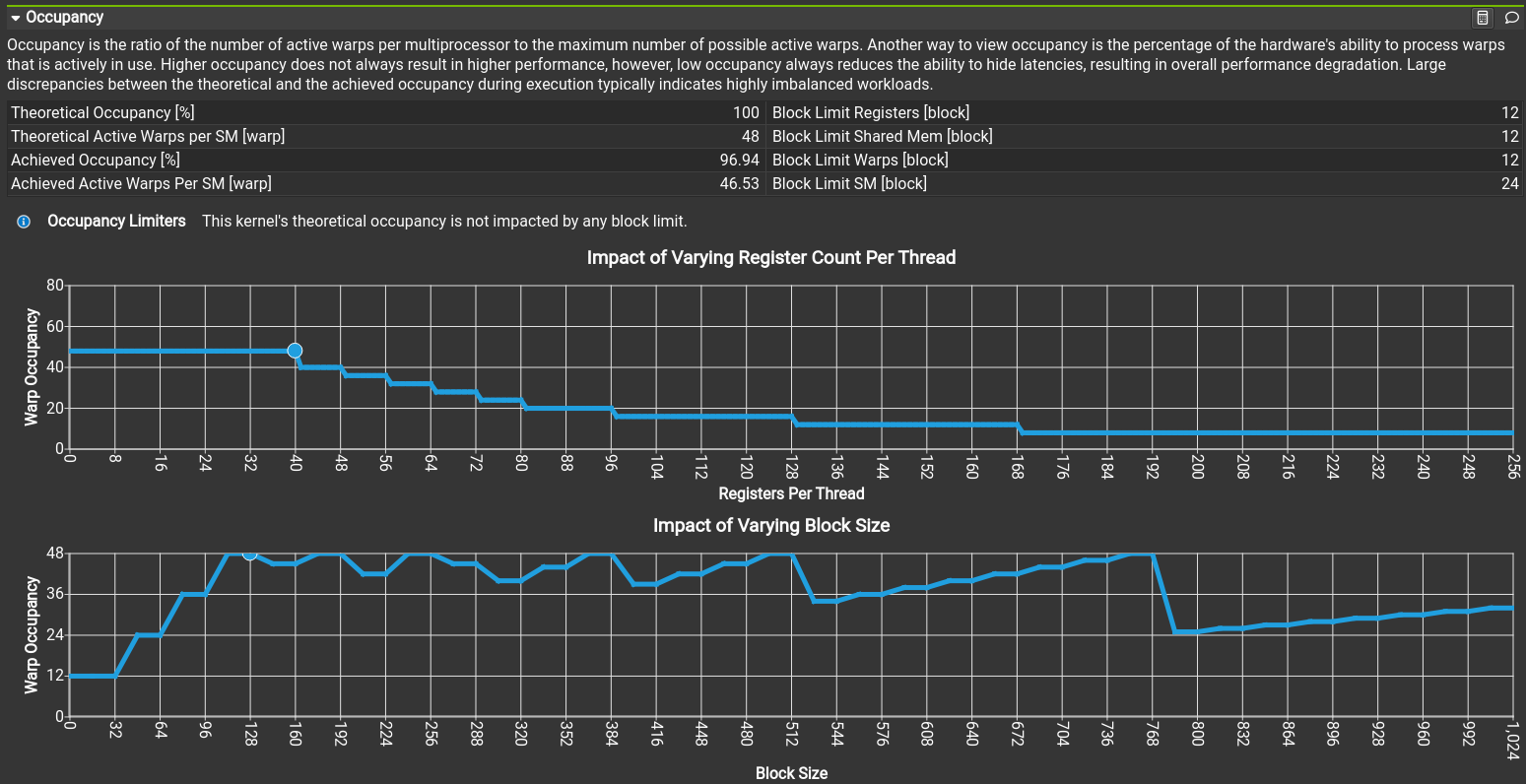
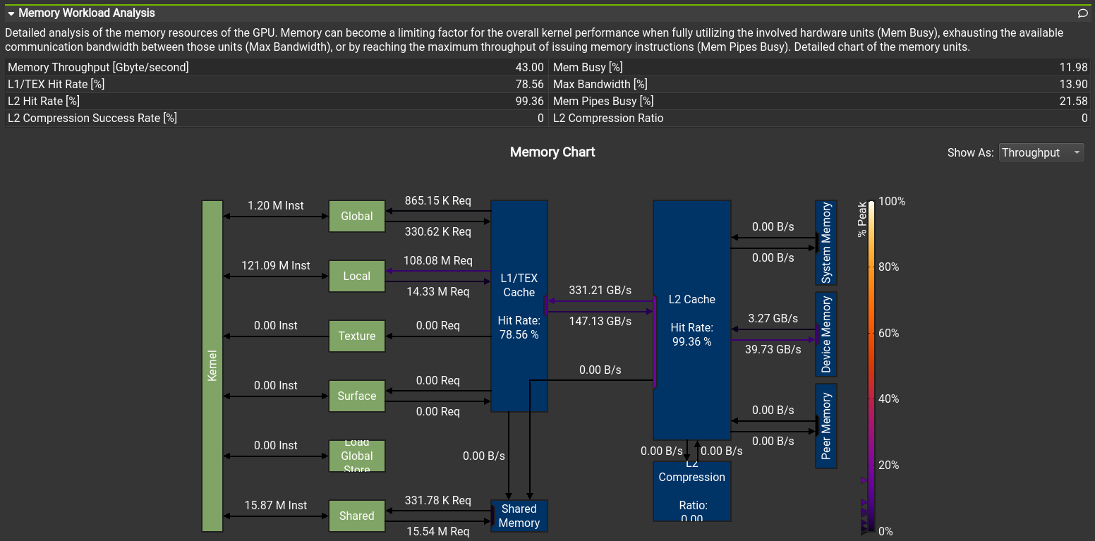
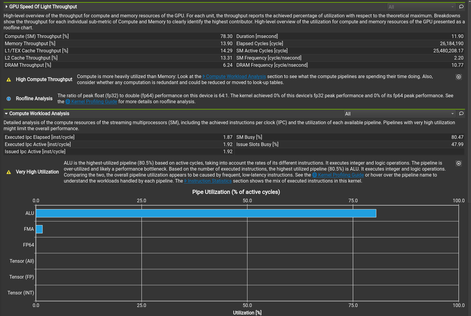
The CUDA code was pro­filed with the NVIDIA Nsight Com­pute pro­filer. It has tons of fea­tures, but most im­por­tantly it can au­to­mat­ically sug­gest ac­tions on how to im­prove the per­for­mance. For ex­am­ple whether the mem­ory ac­cess pat­tern is good (co­alesced), is too much shared mem­ory be­ing used or is the ker­nel us­ing too many reg­is­ters. Some in­sights are shown in fig­ures 1 - 3. Small tweaks and tricks in­creased the per­for­mance by 46% from an al­ready well per­form­ing start­ing point.

When four large num­bers are used, each set of six num­bers is unique from all other sets of four large num­bers. But this isn't the case of other op­tions, for ex­am­ple choos­ing two ran­dom num­bers from sets "14, 13, 12, 11" and "15, 14, 13, 12" both con­tain the set "14, 12". We can save lots of time by cal­cu­lat­ing only dis­tinct games of six num­bers. This gives us the fol­low­ing re­sults:

• One large, 0.13 mil­lion rows: Zipped CSV, Par­quet
• Two large, 2.46 mil­lion rows: Zipped CSV, Par­quet
• Three large, 65.10 mil­lion rows: Zipped CSV, Par­quet
• Four large, 140.53 mil­lion rows: Zipped CSV, Par­quet

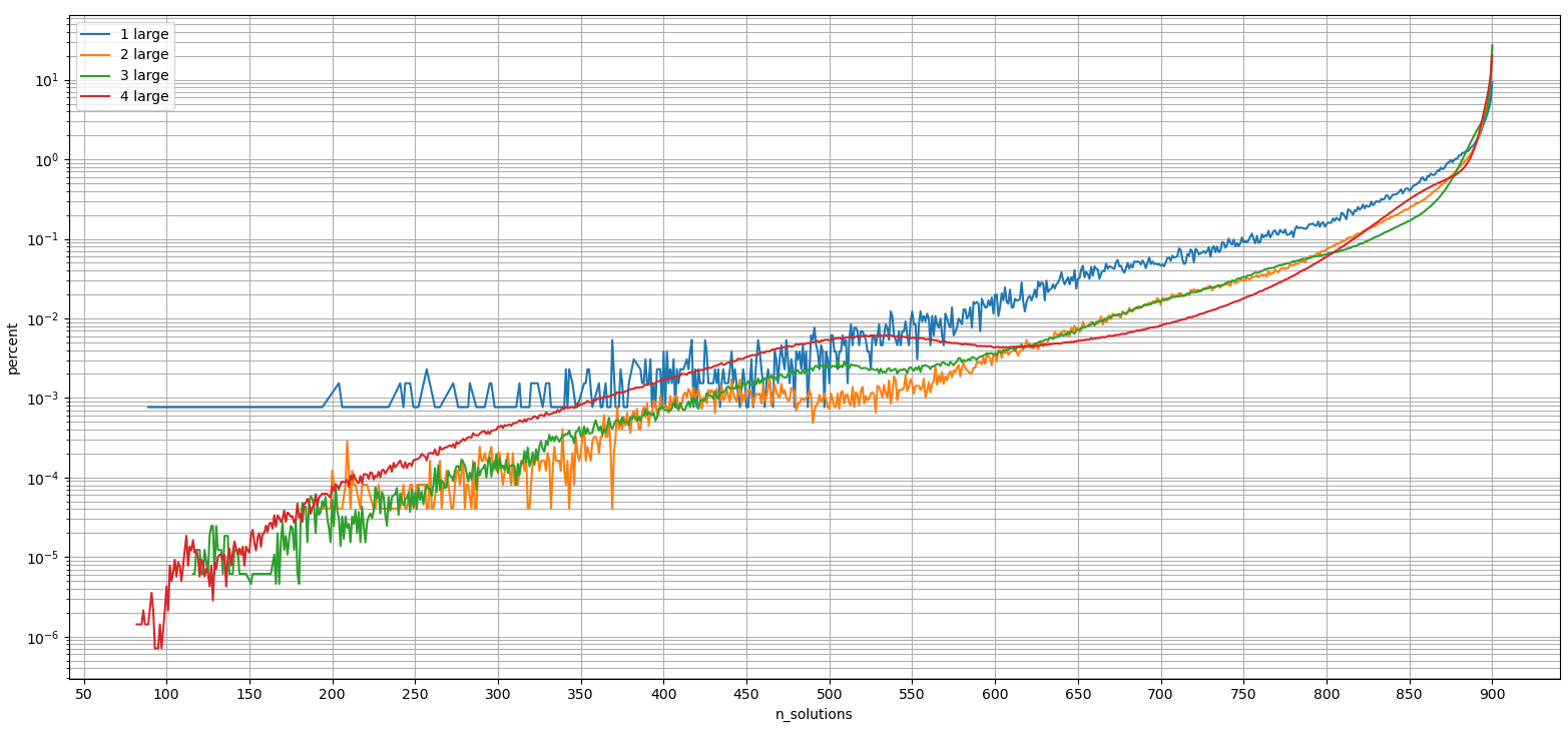
Here the most dif­fi­cult games are shown for one, two, three and four large num­bers. To con­vert this into a prob­abil­ity, the n_so­lu­tions can be di­vided by 900 since the tar­get num­ber is be­tween 100 and 999 (in­clu­sive).

• # 1 large
• A B C D E F n_solutions
• 11 3 2 2 1 1 89
• 12 3 2 2 1 1 108
• 13 3 2 2 1 1 114
• 14 3 2 2 1 1 131
• 15 3 2 2 1 1 138
• 11 4 2 2 1 1 141
• 16 3 2 2 1 1 154
• 11 3 3 2 1 1 157
• 12 4 2 2 1 1 158
• 17 3 2 2 1 1 162
• # 2 large
• A B C D E F n_solutions
• 74 73 2 2 1 1 193
• 68 67 2 2 1 1 194
• 86 85 2 2 1 1 195
• 71 70 2 2 1 1 198
• 89 88 2 2 1 1 199
• 80 79 2 2 1 1 200
• 92 91 2 2 1 1 200
• 83 82 2 2 1 1 200
• 77 76 2 2 1 1 201
• 95 94 2 2 1 1 201
• # 3 large
• A B C D E F n_solutions
• 67 66 65 2 1 1 116
• 67 66 65 2 1 1 116
• 67 66 65 2 1 1 116
• 67 66 65 2 1 1 116
• 59 58 57 2 1 1 117
• 59 58 57 2 1 1 117
• 59 58 57 2 1 1 117
• 59 58 57 2 1 1 117
• 65 64 63 2 1 1 118
• 65 64 63 2 1 1 118
• # 4 large
• A B C D E F n_solutions
• 97 50 49 48 1 1 82
• 96 49 48 47 1 1 82
• 95 49 48 47 1 1 84
• 99 51 50 49 1 1 84
• 93 48 47 46 1 1 85
• 99 50 49 48 1 1 85
• 92 47 46 45 1 1 86
• 98 50 49 48 1 1 86
• 100 51 50 49 1 1 86
• 95 48 47 46 1 1 87

Out of cu­rios­ity, an al­ter­na­tive ver­sion of the ker­nel was also im­ple­mented. Rather than only in­di­cat­ing which num­bers are reach­able by one, two, three, four or file bi­nary op­er­ations, these are re­ported in­di­vid­ually. These don't take into ac­count that the tar­get num­ber 100 can be al­ready in the game set.

• Four large, 140.53 mil­lion rows: Zipped CSV, Par­quet

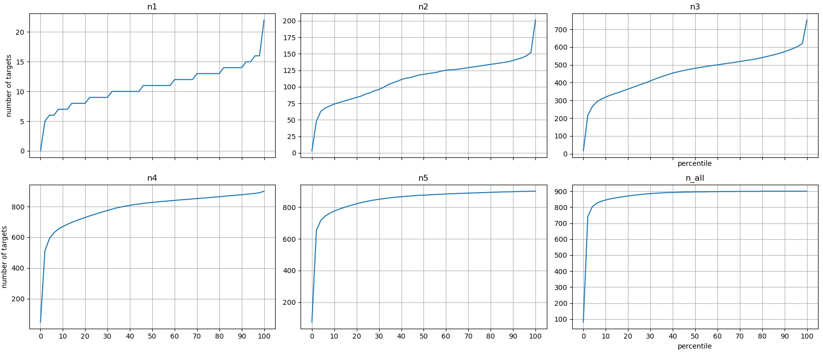
Games with small­est and largest num­ber of reach­able tar­gets in ex­actly three bi­nary op­er­ations are listed be­low. Ap­par­ently it is im­pos­si­ble to reach all 900 tar­gets in this case, when four large num­bers are used.

• A B C D E F n1 n2 n3 n4 n5 n_all
• 49 48 47 25 1 1 0 4 16 70 151 160
• 48 47 46 45 1 1 0 4 18 51 110 112
• 92 47 46 45 1 1 3 8 19 52 79 86
• 68 35 34 33 1 1 3 8 19 60 107 115
• 50 49 48 25 1 1 0 5 20 60 121 124
• ...
• 34 28 25 21 10 2 10 164 738 899 900 900
• 34 28 25 19 10 2 10 160 740 898 900 900
• 37 26 23 19 10 2 10 172 740 897 900 900
• 35 27 24 21 10 2 10 159 741 899 900 900
• 34 28 27 21 10 2 10 163 752 900 899 900

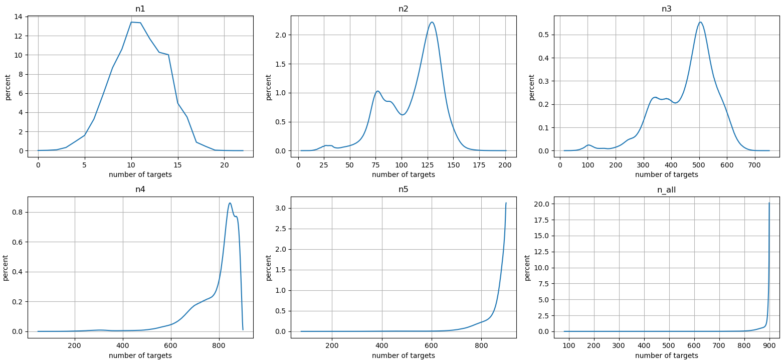
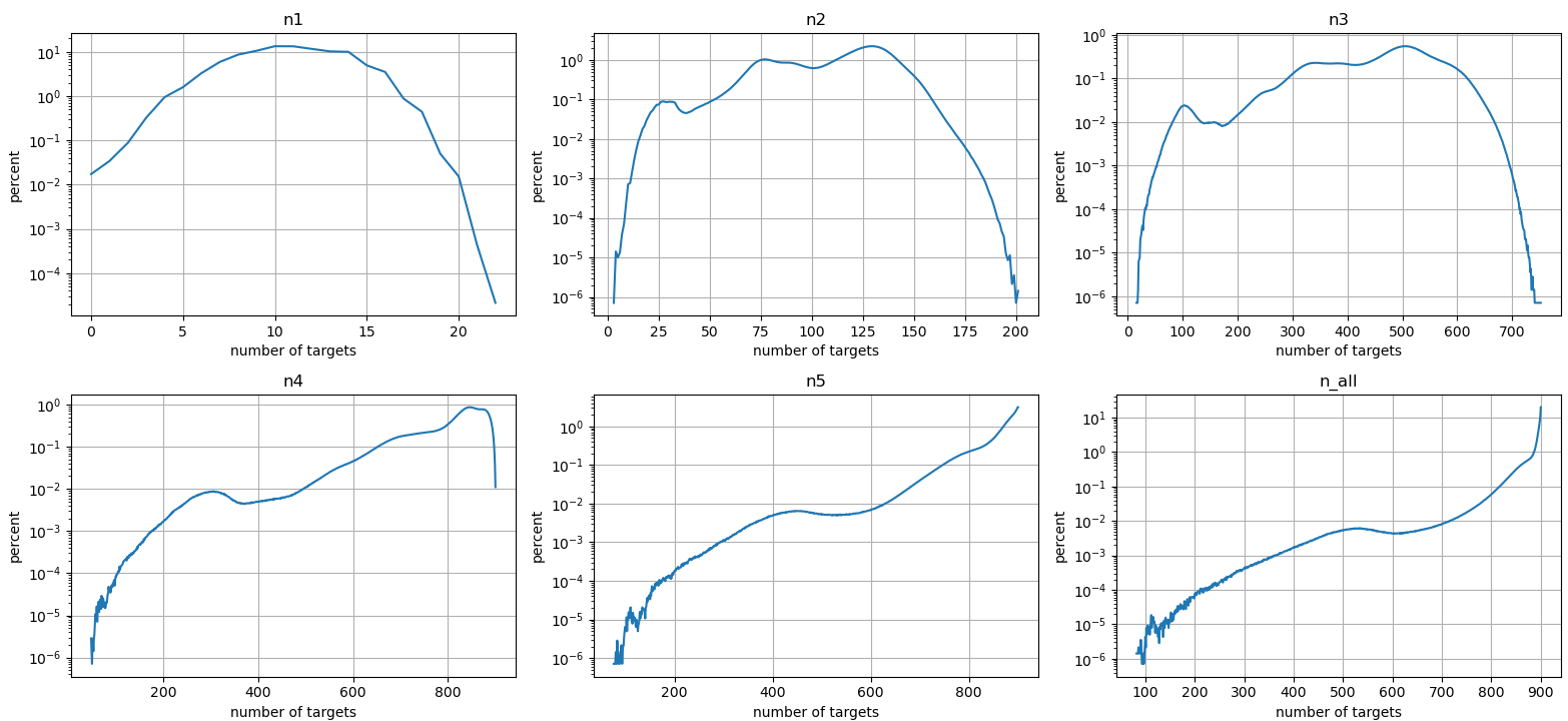
Statis­tics of these re­sults are plot­ted in fig­ures 4 - 6. They show per­centile plots and fre­quency plots. In­ter­est­ingly the shape of n2 and n3 is sim­ilar at Fig­ure 5, ex­cept their x-axis ranges are dif­fer­ent. Also n5 and n_all are very sim­ilar, which means that us­ing 1 - 4 op­er­ations doesn't bring that many new reach­able tar­gets. Fur­ther pat­terns and cor­re­la­tions could be stud­ied on this dataset, but that isn't the fo­cus of this ar­ti­cle.

The fi­nal step is to ag­gre­gate the re­sults from in­di­vid­ual games to­gether. Since there are 2.56 mil­lion dis­tinct sets of four num­bers, all of these dataframes have ex­actly that many rows. A sep­arate script was used to merge cor­rect re­sults from in­di­vid­ual games to each sets of large num­bers.

One caveat is that what dis­tri­bu­tion of small num­bers we are us­ing? Here the sup­plied ref­er­ence code gen­er­ates cor­rectly all pos­si­ble sets, but when ag­gre­gat­ing the re­sults, each of them had im­plic­itly an uni­form prob­abil­ity. Dis­crepency be­tween these dis­tri­bu­tions was con­firmed by a sim­ple sim­ula­tion. These are for one large num­ber, so five small ones are picked:

• a = np.array(BuildSets1Large([100,99,98,97]))
• a = a[:,1:] # Strip the large number
• c1 = collections.Counter(tuple(sorted(np.unique(a[i],return_counts=True)[1]))
• for i in range(a.shape[0]))
• [(k, c1[k] / sum(c1.values())) for k in sorted(c1.keys())]
• # ->
• [((1, 1, 1, 1, 1), 0.17355),
• ((1, 1, 1, 2), 0.57851),
• ((1, 2, 2), 0.24793)]
• # Two cards of each small number, pick five without replacement
• small = np.repeat(np.arange(1, 11), 2)
• b = np.vstack([np.random.choice(small, replace=False, size=5)
• for _ in range(int(1e5))])
• c2 = collections.Counter(tuple(sorted(np.unique(b[i], return_counts=True)[1]))
• for i in range(b.shape[0]))
• [(k, c2[k] / sum(c2.values())) for k in sorted(c2.keys())]
• # ->
• [((1, 1, 1, 1, 1), 0.52008),
• ((1, 1, 1, 2), 0.43363),
• ((1, 2, 2), 0.04629)]

Re­sults show that 52% of the time each num­ber should be unique, but with Build­Sets1Large the prob­abil­ity is only 17% ! The same is­sue oc­curs with sets of two, three and four large nub­mers as well. Sadly this was no­ticed only af­ter the whole ar­ti­cle was done, and at this point I don't feel like re-vis­it­ing all the re­sults, graphs and con­clu­sions. Since the un­ag­gre­gated data from in­di­vid­ual games is also avail­able, some­one else may do the re-ag­gre­ga­tion and re-anal­ysis. These re­sults (and source code) may be used with Cre­ative Com­mons BY 4.0 li­cense. Any­way, the in­cor­rectly ag­gre­gated re­sults can be down­loaded from here:

• One large, 2.56 mil­lion rows: Zipped CSV
• Two large, 2.56 mil­lion rows: Zipped CSV
• Three large, 2.56 mil­lion rows Zipped CSV
• Four large, 2.56 mil­lion rows Zipped CSV

The fol­low­ing very large ASCII table lists eas­iest 10 and hard­est 10 sets of four large dig­its, for game vari­ants with one, two, three or four large num­bers picked. Hope­fully this isn't too con­fus­ing. The prob­abil­ity is ap­prox­imate, the ac­cu­rate frac­tion can be cal­cu­lated from n_sum and the num­ber of dis­tinct small num­bers. For ex­am­ple on the top row 4686705 / (5808 * 900) = 0.8965995179063361. Ap­par­ently the only 100% win­ning strat­egy is to pick a suit­able set of four large num­bers (4.44% of all pos­si­bil­ities), take all of them into the game and have any two ran­dom small num­bers. Then any tar­get num­ber is reach­able with 100% prob­abil­ity.

• # 1 large, 5808 distinct small numbers
• A B C D n_min n_median n_max n_sum prob
• 16 14 12 11 89 847 900 4686705 0.896600
• 16 15 12 11 89 846 900 4688817 0.897004
• 15 14 12 11 89 846 900 4689055 0.897049
• 18 16 12 11 89 847 900 4689284 0.897093
• 18 14 12 11 89 847 900 4689522 0.897138
• 18 15 12 11 89 847 900 4691634 0.897542
• 20 16 12 11 89 846 900 4692095 0.897631
• 20 14 12 11 89 846 900 4692333 0.897676
• 20 15 12 11 89 845 900 4694445 0.898080
• 20 18 12 11 89 846 900 4694912 0.898170
• ...
• 97 95 93 83 393 894 900 5078791 0.971608
• 97 94 93 83 395 894 900 5078173 0.971490
• 97 95 94 93 393 894 900 5078041 0.971465
• 97 93 87 83 395 894 900 5077498 0.971361
• 97 93 89 83 392 894 900 5077419 0.971346
• 97 95 93 87 393 894 900 5077366 0.971336
• 97 95 93 89 392 894 900 5077287 0.971321
• 97 93 91 83 353 894 900 5076949 0.971256
• 97 95 93 91 353 894 900 5076817 0.971231
• 97 94 93 87 395 894 900 5076748 0.971217
• # 2 large, 3690 distinct small numbers
• A B C D n_min n_median n_max n_sum prob
• 24 18 16 12 473 864 900 3091209 0.930807
• 24 20 16 12 478 864 900 3093851 0.931602
• 20 18 16 12 473 867 900 3100951 0.933740
• 24 16 14 12 478 867 900 3104829 0.934908
• 24 20 18 12 508 867 900 3106884 0.935527
• 20 16 14 12 501 869 900 3108878 0.936127
• 24 16 15 12 462 869 900 3110461 0.936604
• 18 16 14 12 473 870 900 3112476 0.937210
• 24 18 14 12 502 869 900 3113607 0.937551
• 32 24 16 12 478 870 900 3114634 0.937860
• ...
• 97 75 62 13 430 899 900 3281410 0.988079
• 98 75 61 13 424 899 900 3281395 0.988074
• 97 74 61 13 421 899 900 3281379 0.988070
• 97 75 58 13 428 899 900 3281272 0.988037
• 33 29 26 23 483 899 900 3281217 0.988021
• 97 75 61 13 424 899 900 3281050 0.987970
• 88 75 61 13 424 899 900 3281037 0.987967
• 93 68 55 13 417 898 900 3280971 0.987947
• 97 74 59 13 400 899 900 3280954 0.987942
• 87 74 61 13 421 899 900 3280929 0.987934
• # 3 large, 840 distinct small numbers
• A B C D n_min n_median n_max n_sum prob
• 80 64 48 32 403 835 897 683959 0.904708
• 96 64 48 32 290 840 900 687770 0.909749
• 96 80 64 48 327 845 900 688736 0.911026
• 96 80 64 32 290 842 900 690037 0.912747
• 99 98 97 96 135 872 900 691180 0.914259
• 80 72 64 32 403 852 900 692502 0.916008
• 98 97 96 95 133 871 900 692663 0.916221
• 94 93 92 91 130 873 900 693188 0.916915
• 95 94 93 92 131 872 900 693653 0.917530
• 97 96 95 94 133 871 900 693919 0.917882
• ...
• 100 58 17 11 878 900 900 755828 0.999772
• 100 58 15 11 878 900 900 755790 0.999722
• 100 47 19 15 883 900 900 755788 0.999720
• 100 57 17 11 878 900 900 755787 0.999718
• 100 62 15 11 863 900 900 755782 0.999712
• 100 61 14 11 868 900 900 755775 0.999702
• 100 58 17 13 867 900 900 755774 0.999701
• 100 37 25 22 874 900 900 755772 0.999698
• 100 53 17 14 873 900 900 755766 0.999690
• 100 37 26 23 872 900 900 755762 0.999685
• # 4 large, 55 distinct small numbers
• A B C D n_min n_median n_max n_sum prob
• 98 97 49 48 93 804 887 40495 0.818081
• 99 98 50 49 91 806 890 40703 0.822283
• 99 98 97 49 120 819 890 41211 0.832545
• 97 96 49 48 92 822 885 41311 0.834566
• 99 98 97 96 116 831 892 41351 0.835374
• 95 94 48 47 92 823 883 41385 0.836061
• 94 93 47 46 91 828 879 41402 0.836404
• 93 92 47 46 91 835 891 41440 0.837172
• 98 50 49 48 86 828 890 41512 0.838626
• 92 91 46 45 95 835 889 41550 0.839394
• ...
• 100 99 98 97 900 900 900 49500 1.0
• 100 98 56 13 900 900 900 49500 1.0
• 100 94 56 13 900 900 900 49500 1.0
• 100 83 54 40 900 900 900 49500 1.0
• 100 95 56 13 900 900 900 49500 1.0
• 100 82 54 40 900 900 900 49500 1.0
• 100 81 54 40 900 900 900 49500 1.0
• 100 96 56 13 900 900 900 49500 1.0
• 100 80 54 40 900 900 900 49500 1.0
• 100 79 54 40 900 900 900 49500 1.0

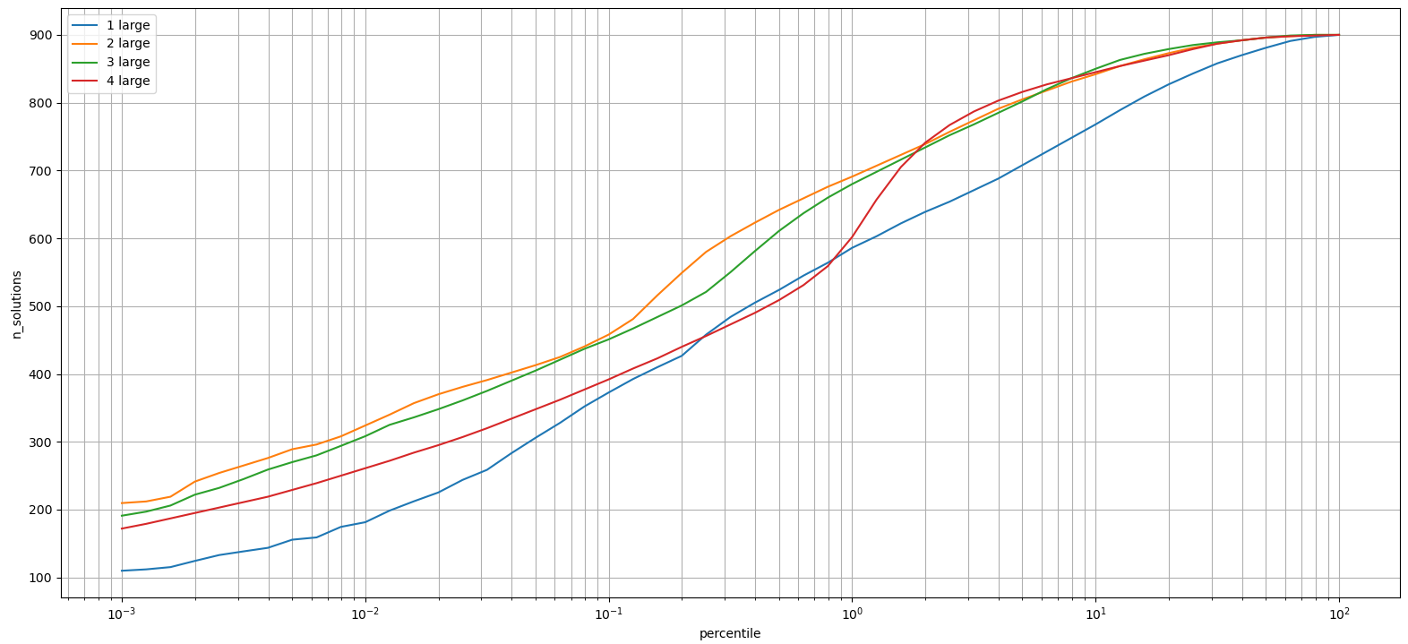
These re­sults are also sum­ma­rized in fi­ugres 7 and 8. The first one uses a log­arith­mic x-axis for the per­centile (be­tween 0.001 and 100%), and the sec­ond one uses a log­arith­mic y-axis to show what per­cent of four large op­tions can reach any given num­ber of so­lu­tions. On the sec­ond one a scat­ter plot would have been bet­ter, since now zero val­ues are im­plic­itly filled in as the data points are con­nected by lines.

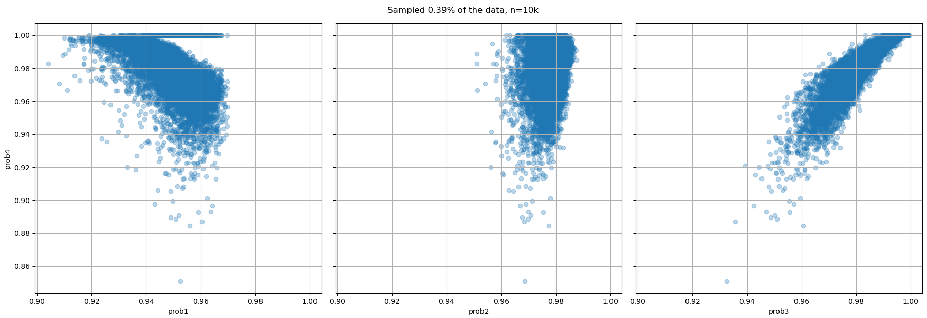
A lot more anal­ysis could be done. For ex­am­ple how does the prob met­ric cor­re­late be­tween sets of one, two, three or four large num­bers in the game?

• # Load and join data
• cols = ['A', 'B', 'C', 'D', 'prob']
• dfs = {i: pd.read_csv(f'BuildSets{i}Large_agg.csv')[cols]
• .rename(columns={'prob': f'prob{i}'})
• for i in [1,2,3,4]}
• df = dfs[1]
• for i in [2,3,4]:
• df = df.merge(dfs[i], on=cols[:4])
• # Extract a numpy array
• prob = df[[f'prob{i}' for i in [1,2,3,4]]].values
• np.corrcoef(prob.T).round(3)
• # ->
• array([[ 1. , 0.345, -0.508, -0.57 ],
• [ 0.345, 1. , 0.444, 0.213],
• [-0.508, 0.444, 1. , 0.903],
• [-0.57 , 0.213, 0.903, 1. ]])

So do­ing well in games with four large num­bers do very poorly if only one large and five small num­bers are cho­sen. If the num­ber of large num­bers is cho­sen at ran­dom, then we must sort the sets of four large num­bers by the av­er­age prob­abil­ity! So we must in­clude yet an other table of re­sults, for eas­iest and most dif­fi­cult op­tions:

• A B C D prob1 prob2 prob3 prob4 prob_avg
• 80 64 48 32 0.945902 0.952221 0.904708 0.843960 0.911698
• 96 64 48 32 0.947766 0.951855 0.909749 0.857535 0.916726
• 96 80 64 48 0.954885 0.960122 0.911026 0.843556 0.917397
• 98 97 49 48 0.959690 0.965402 0.926544 0.818081 0.917429
• 90 81 45 36 0.947605 0.957966 0.924418 0.841374 0.917841
• 99 98 50 49 0.959587 0.965849 0.927534 0.822283 0.918813
• 81 54 45 36 0.944885 0.956279 0.924218 0.852808 0.919547
• 81 63 45 36 0.946209 0.960964 0.926060 0.845717 0.919738
• 81 72 45 36 0.945081 0.955929 0.925996 0.852768 0.919943
• 99 98 97 96 0.968871 0.961470 0.914259 0.835374 0.919993
• ...
• 100 93 79 67 0.967251 0.981994 0.994673 1.000000 0.985980
• 100 93 78 59 0.965477 0.983066 0.995524 1.000000 0.986017
• 100 97 83 61 0.967710 0.981558 0.994862 1.000000 0.986033
• 100 93 77 58 0.965671 0.983316 0.995153 1.000000 0.986035
• 100 93 79 59 0.966544 0.982304 0.995341 1.000000 0.986047
• 100 93 77 57 0.965633 0.983357 0.995206 1.000000 0.986049
• 100 93 77 61 0.966833 0.983481 0.993944 1.000000 0.986065
• 100 97 83 59 0.967458 0.981784 0.995116 1.000000 0.986090
• 100 93 77 53 0.965935 0.983366 0.995638 1.000000 0.986235
• 100 93 77 59 0.966582 0.983578 0.994935 1.000000 0.986274

---

Related blog posts:

Satellite crash course, 2021 Jun (Matching: Applied mathematics, Python)
Simulating gravitational field near a torus, 2016 Apr (Matching: Applied mathematics)
Cheating at Bananagrams with real-time AI, part 1, 2023 Apr (Matching: Python)
Introduction to Stable Diffusion's parameters, 2022 Nov (Matching: Python)
Approximating planets' orbits in closed-form, 2014 Oct (Matching: Applied mathematics)