Niko's Project Corner

---

Ba­nana­grams is a real-time word game in which par­tic­ipants race to build their own cross­words. It re­quires com­pre­hen­sive vo­cab­ulary, fast think­ing and good de­ci­sion mak­ing. Some times sit­ua­tions arise which re­quire an ei­ther-or de­ci­sion: do I scrap my par­tial so­lu­tion and do a fresh start or not? Or you may be left with one un­us­able ex­tra let­ter, which you can put back into the pile and pick up three ran­dom new ones. This first ar­ti­cle of the topic de­scribes a two-phase ar­ti­fi­cial neu­ral net­work which de­tects and iden­ti­fies the tiles from an im­age. The sec­ond ar­ti­cle will de­scribe how to gen­er­ate a valid cross­word from given let­ters.

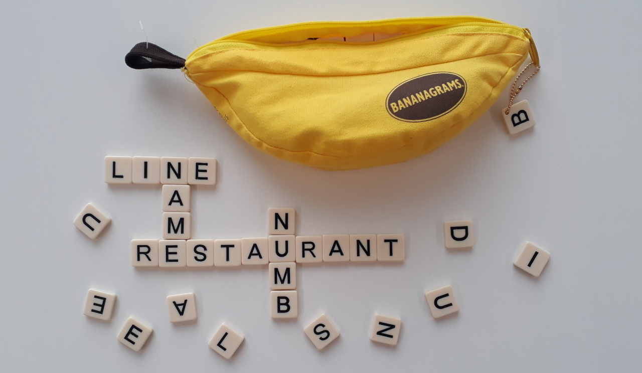
An ex­am­ple game set is shown in Fig­ure 1. There are a few dif­fer­ent rule-sets, but in one of them each player is dealth N ran­dom tiles face down, and when ev­ery­body is ready, they are flipped over and it is just a race to con­struct a valid cross­word which uses all the tiles.

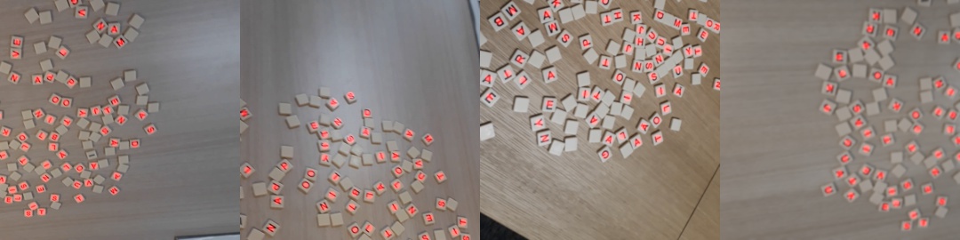
The first step is to lo­cal­ize tiles from a given im­age. The train­ing data was con­structed by sim­ply man­ually cre­at­ing a black-and-white mask in GIMP, in which a pixel is white if it is near the cen­ter of a tile, or black if it is not. An ex­am­ple is shown in Fig­ure 2.

Source videos have a res­olu­tion of 1920 × 1080, which are down­scaled to 25% of the orig­inal size to a res­olu­tion of 480 × 270. Each frame's two halves are used as two sep­arate sam­ples, and the net­work is trained on rect­an­gu­lar im­ages of res­olu­tion 270 × 270. The net­work could be trained with non-rect­an­gu­lar im­ages as well, but data aug­men­ta­tion (es­pe­cially im­age ro­ta­tions) work bet­ter on rect­an­gu­lar ones.

Each sam­ple is used to gen­er­ate four ver­sions of it, ap­ply­ing ro­ta­tions by 0, 90, 180 and 270 de­grees and also in­tro­duc­ing gaus­sian blur with a ran­dom ra­dius. Since there are 21 frames of train­ing data, the shape of the Numpy ar­ray is 21 * 2 * 4 × 270 × 270 × 4 = 168 × 270 × 270 × 4. The last three di­men­sions are in­put im­age's red, green and blue val­ues, and the fouth one is the in­tended mask. Ex­am­ples are shown in Fig­ure 3, where the last chan­nel is com­bined with the in­put im­age's red chan­nel.

The tile de­tec­tion net­work uses only 2D con­vo­lu­tions and batch nor­mal­iza­tion, so in the fully in­te­grated ap­pli­ca­tion it can be used di­rectly on the 480 × 270 re­olu­tion frame. There are many hy­per­pa­ram­eters to ad­just (the num­ber of stacked lay­ers, num­ber of ker­nels, amount of dropout, ...), but rea­son­able loss (bi­nary cross en­tropy) and ac­cu­racy was ob­tained with the fol­low­ing struc­ture. In the fi­nal ap­pli­ca­tion also real-time per­for­mance goal needs to be taken into ac­count.

Here we can see that the res­olu­tion drops from 270 to 258 pix­els, or by 12 pix­els. This means that the de­ci­sion on whether an out­put pixel be­longs to a tile's cen­ter or not is done on a re­gion of in­ter­est of ±6 pix­els, or in other words 13 × 13 pix­els. Tak­ing the down­scal­ing by 1:4 into ac­count, this cor­re­sponds to ±24 or 49 × 49 pix­els in the FullHD frame.

• Layer (type) Output Shape Param #
• =================================================================
• (None, 270, 270, 3) 0
• conv2d_6 (Conv2D) (None, 268, 268, 16) 448
• batch_normalization_5 (Batch (None, 268, 268, 16) 64
• conv2d_7 (Conv2D) (None, 266, 266, 10) 1450
• batch_normalization_6 (Batch (None, 266, 266, 10) 40
• conv2d_8 (Conv2D) (None, 264, 264, 10) 910
• batch_normalization_7 (Batch (None, 264, 264, 10) 40
• conv2d_9 (Conv2D) (None, 262, 262, 10) 910
• batch_normalization_8 (Batch (None, 262, 262, 10) 40
• conv2d_10 (Conv2D) (None, 260, 260, 10) 910
• batch_normalization_9 (Batch (None, 260, 260, 10) 40
• conv2d_11 (Conv2D) (None, 258, 258, 1) 91
• =================================================================
• Total params: 4,943
• Trainable params: 4,831
• Non-trainable params: 112
• _________________________________________________________________

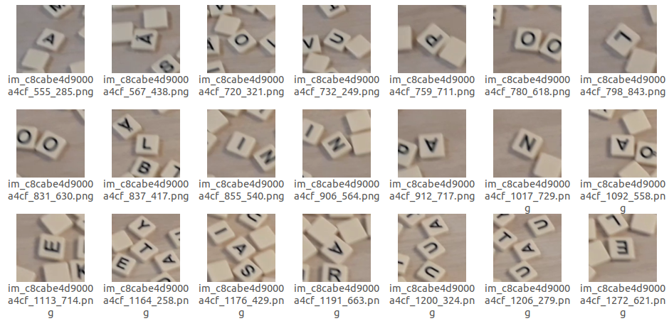
Once the de­tec­tion layer is trained, it can be used to ex­tract in­di­vid­ual tiles from videos. Im­age re­gions are cropped at ±64 pix­els from the cen­ter, re­sult­ing in im­ages of res­olu­tion 128 × 128. Ex­am­ples of these are shown in Fig­ure 4. Note that there are sev­eral as­pects which make this clas­si­fi­ca­tion task non-triv­ial:

• Cam­era's dis­tance from the table isn't con­trolled, mean­ing that the let­ters may ap­pear larger or smaller.
• The point of view isn't con­strained to be top-down, mean­ing that there are dis­tor­tion caused by per­spec­tive
• Tile's ori­en­ta­tion is ran­dom, but still let­ters with sim­ilar struc­ture such as A and V must be dis­tin­guished. And don't for­get about Ä!
• Tiles are scat­tered on the table and not neatly sep­arated, mean­ing that the net­work must learn to fo­cus only on the tile on the mid­dle of the im­age.
• Low light con­di­tion and cam­era mo­tion cause noise and blur ef­fects on im­ages.

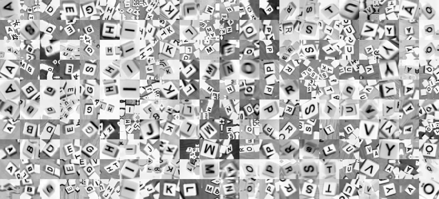
The iden­ti­fi­ca­tion net­work is trained us­ing black and white im­ages. The raw dataset con­sists of 4500 man­ually la­beled im­ages, with vary­ing num­ber of ex­am­ples per class. The small­est one is G (49 im­ages) and the most com­mon is A (455 im­ages). It should be noted that a Finnish ver­sion of the game was used, so let­ters like G, B and D are relatively rare and C is totally absent. Naturally image augmentation (random rotation, crop, noise, blur, ...) is used to extend the dataset. In the training and validation datasets each class had equal frequency, for example 5k or 20k samples per class. Examples are shown in Figure 5. Training is done on images rescaled to just 64 × 64 pixels, since this resulted in sufficient accuracy and is faster in the intended real-time application.

The net­work could be di­rectly trained on "raw" un­pro­cessed im­ages, but bet­ter ac­cu­racy was ob­tained by co-train­ing a pre-pro­cess­ing model si­mul­ta­ne­ously with the ac­tual clas­si­fi­ca­tion model. The task of the pre-pro­cess­ing model is to mask out ir­rel­evant other let­ters near the im­age bor­der, and op­tion­ally also in­crease the global con­trast. The fol­low­ing net­work takes a sub-sam­pled 64 × 64 im­age and out­puts ei­ther one or two pre­dicted val­ues, de­pend­ing whether also the bright­ness is ad­justed. The first out­put is the cen­tral let­ter's es­ti­mated ra­dius (nor­mal­ized to 0 - 1), and the sec­ond one is the amount of bright­ness to add. It has only a few thou­sand pa­ram­eters, and seems to be work­ing just fine.

• Layer (type) Output Shape Param #
• =================================================================
• (None, 64, 64, 1) 0
• conv2d_12 (Conv2D) (None, 60, 60, 16) 416
• max_pooling2d (MaxPooling2D) (None, 20, 20, 16) 0
• batch_normalization_10 (Batc (None, 20, 20, 16) 64
• conv2d_13 (Conv2D) (None, 18, 18, 6) 870
• max_pooling2d_1 (MaxPooling2 (None, 6, 6, 6) 0
• batch_normalization_11 (Batc (None, 6, 6, 6) 24
• conv2d_14 (Conv2D) (None, 4, 4, 6) 330
• batch_normalization_12 (Batc (None, 4, 4, 6) 24
• flatten (Flatten) (None, 96) 0
• dense (Dense) (None, 6) 582
• batch_normalization_13 (Batc (None, 6) 24
• dense_5 (Dense) (None, 2) 14
• =================================================================
• Total params: 2,348
• Trainable params: 2,280
• Non-trainable params: 68
• _________________________________________________________________

Us­ing the pre-pro­cess­ing model is a bit non-triv­ial, it doesn't use the Se­quen­tial in­ter­face but in­stead the more generic Model one. It pre-cal­cu­lates a "ra­dius" ten­sor mr, with a dis­tance value of zero in the mid­dle and √2  in all cor­ners, mean­ing that the used co­or­di­nate grid is from a range of -1 — 1 (from vari­ables mx and my). The sig­moid ac­ti­va­tion is used in a man­ner which causes the added bright­ness to be zero in the im­age cen­ter, and one out­side the es­ti­mated ra­dius. Here some care needs to be taken, so that Ten­sor­flow can ap­ply proper broad­cast­ing be­tween these mis-matched ten­sors. And one must re­mem­ber that the first ze­roth di­men­sion is NOT im­age's height, is the batch size!

If the out­put rx from the pre-pro­cess­ing model has more than one out­put, the sec­ond out­put is added to the im­age. Pix­els are then clipped be­tween val­ues of zero and one, ba­si­cally sat­urat­ing the max­imum bright­ness. Im­age is then re-nor­mal­ized so that its min­imum value is al­ways zero. The max­imum bright­ness could be smaller than one though. This source code is syn­tax-high­lighted nicer on the PDF ver­sion.

• import tensorflow.keras.layers as l
• from tensorflow.keras.models import Model
• import tensorflow.keras.backend as K
• import numpy as np
• res = 64
• mx, my = np.meshgrid(*(np.linspace(-1, 1, res) for _ in range(2)))
• mr = tf.cast(((mx**2 + my**2)**0.5)[None,:,:,None], dtype=tf.float32)
• inp = l.Input(X_fit.shape[1:])
• rx = r_model(inp)
• # Add brightness outside the radius
• x = inp + K.sigmoid((mr - rx[:,0:1,None,None]) * 10)
• # Optionally increase the global brightness as well
• if rx.shape[1] > 1:
• x = x + rx[:,1:2,None,None]
• # Clip the brightness, re-scale the values so
• # that the darkest pixel has a value of zero
• x = K.clip(x, 0, 1)
• x_min = K.min(x, axis=(1,2))[:,:,None,None]
• x = (x - x_min) / (1 - x_min + K.epsilon())
• m_model = Model(inp, x)

The com­plete model is eas­ily con­structed with the Se­quen­tial in­ter­face, and it can in­cor­po­rate the pre-pro­cess­ing model with­out any is­sues. There are quite many hy­per­pa­ram­eters to choose from, but this re­sulted in a fairly good ac­cu­racy. The model has about 80k para­maters, start­ing with typ­ical Conv2D, BatchNormalization, SpatialDropout2D and MaxPooling2D layers and finishing up with fully connected Dense layers.

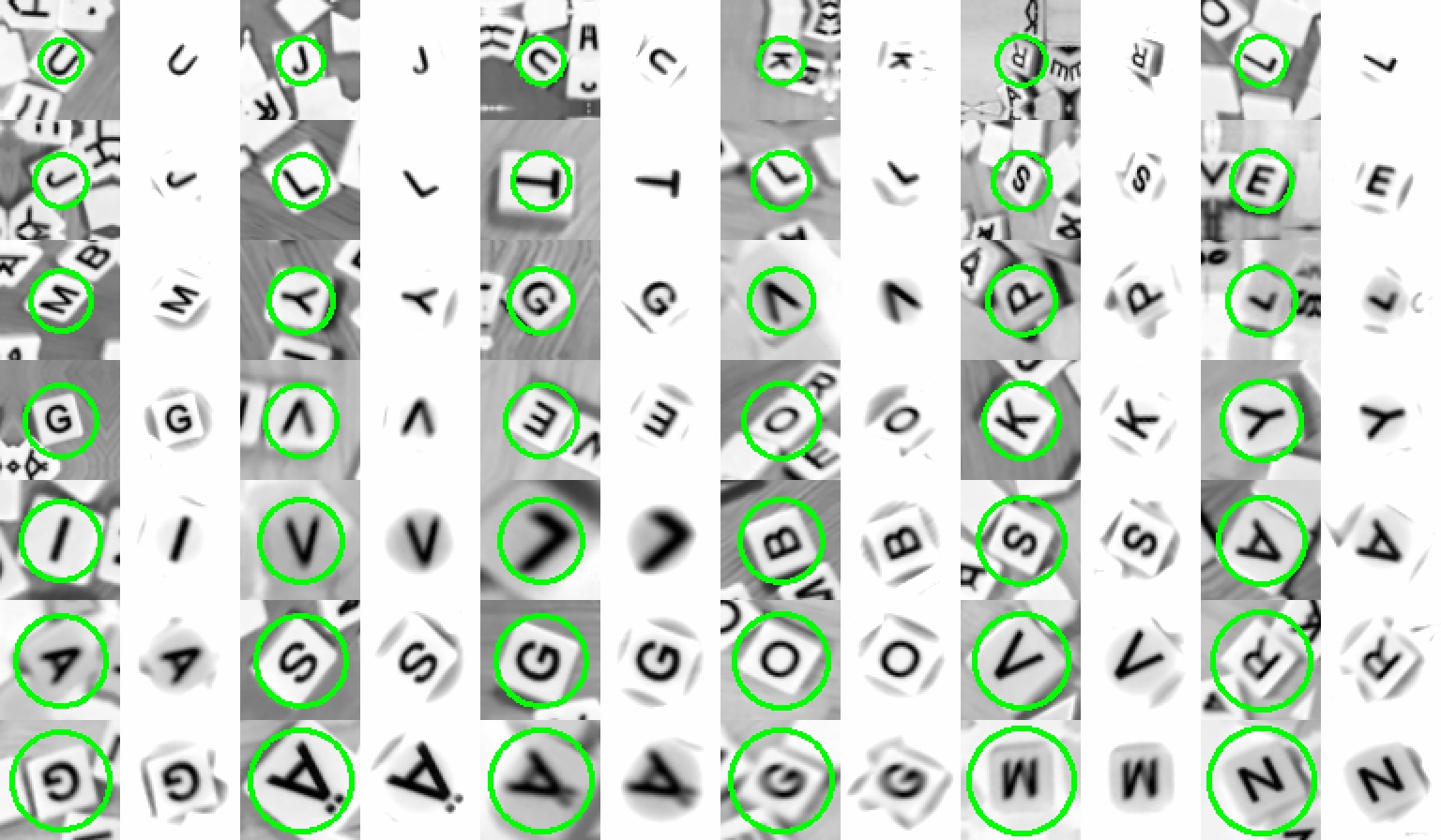
It was a bit sur­pris­ing that the pre-pro­cess­ing model worked out so well, even with to­tally ran­dom ini­tial­iza­tion and no ex­plicit in­for­ma­tion on the cor­rect ra­dius. It just learned that es­pe­cially when the cam­era was far away and the cen­tral let­ter cov­ers just a small part of the im­age, it is im­por­tant to mask out all ex­tra let­ters so that they don't con­fuse the deeper lay­ers. Es­ti­mated radii and pre-pro­cessed im­ages are shown in Fig­ure 6, sorted from small­est to largest. Bound­ing cir­cles aren't 100% tight, but here a high pre­ci­sion isn't re­quired.

• Layer (type) Output Shape Param #
• =================================================================
• (None, 64, 64, 1) 0
• model_1 (Functional) (None, 64, 64, 1) 2348
• conv2d_21 (Conv2D) (None, 62, 62, 48) 480
• max_pooling2d_7 (MaxPooling2 (None, 31, 31, 48) 0
• spatial_dropout2d_3 (Spatial (None, 31, 31, 48) 0
• batch_normalization_22 (Batc (None, 31, 31, 48) 192
• conv2d_22 (Conv2D) (None, 28, 28, 48) 36912
• max_pooling2d_8 (MaxPooling2 (None, 14, 14, 48) 0
• spatial_dropout2d_4 (Spatial (None, 14, 14, 48) 0
• batch_normalization_23 (Batc (None, 14, 14, 48) 192
• conv2d_23 (Conv2D) (None, 12, 12, 48) 20784
• max_pooling2d_9 (MaxPooling2 (None, 4, 4, 48) 0
• spatial_dropout2d_5 (Spatial (None, 4, 4, 48) 0
• batch_normalization_24 (Batc (None, 4, 4, 48) 192
• flatten_3 (Flatten) (None, 768) 0
• dense_6 (Dense) (None, 22) 16918
• batch_normalization_25 (Batc (None, 22) 88
• dense_7 (Dense) (None, 22) 506
• =================================================================
• Total params: 78,612
• Trainable params: 78,212
• Non-trainable params: 400
• _________________________________________________________________

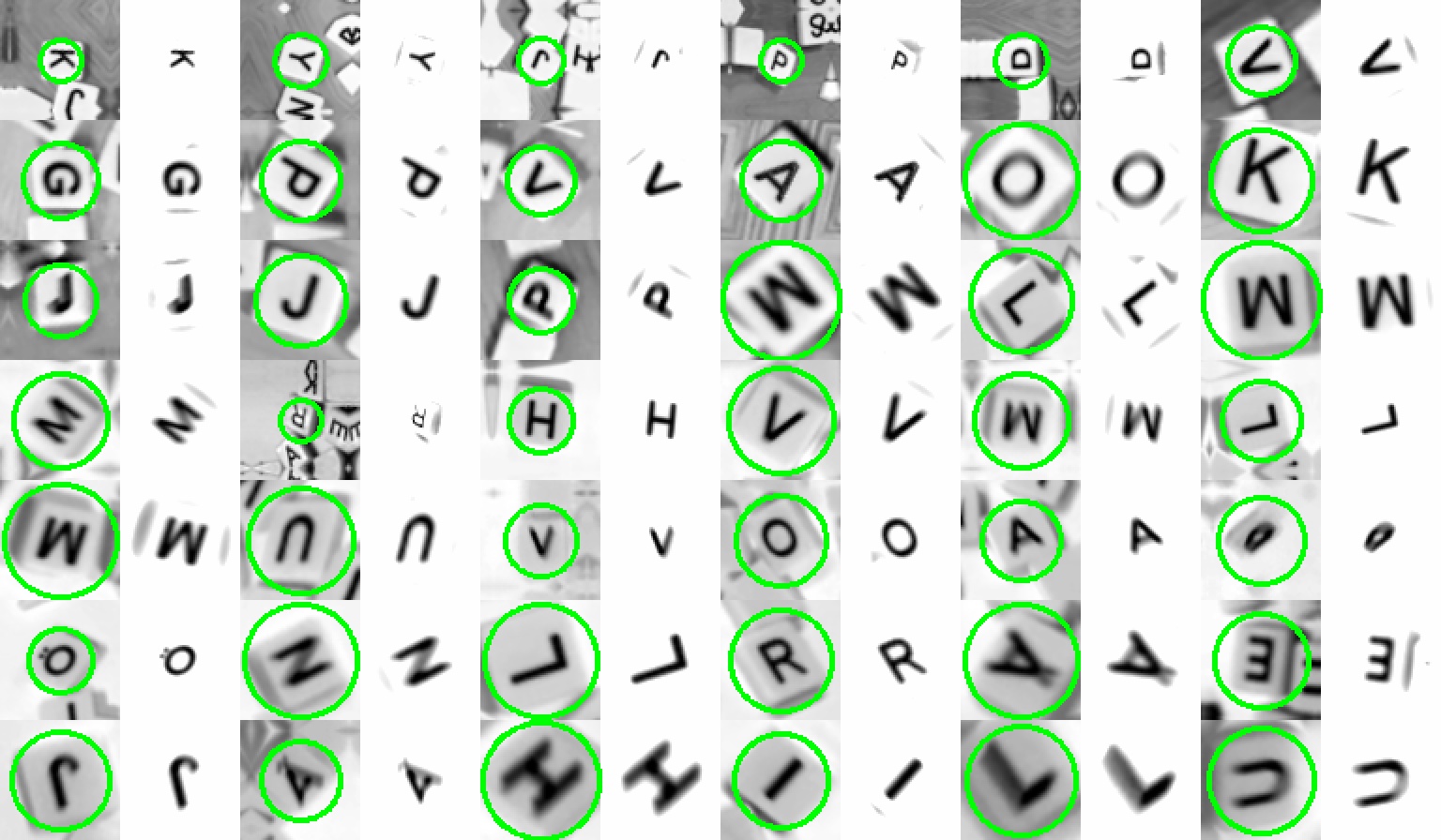
Es­ti­mated radii and op­ti­mal bright­nesses are shown in Fig­ure 7. Note that un­like in Fig­ure 6, in 7 im­ages are sorted by the amount of added brigth­ness. This means that the let­ter K on top left has the least amount of ex­tra brigth­ness (it be­ing al­ready on a very bright back­ground, and a cor­rectly es­ti­mated bound­ing cir­cle), and the U on bot­tom right had the dark­est back­ground. The re­sult­ing im­ages have very few ex­tra arte­facts, ex­cept the square tile's shadow in some cases.

Class ac­cu­ra­cies and con­fu­sion ma­tri­ces for fit and val­ida­tion data are shown in fig­ures 8 and 9. The con­fu­sion ma­trix has a white column for let­ters which were iden­ti­fied cor­rectly 100% of the time.

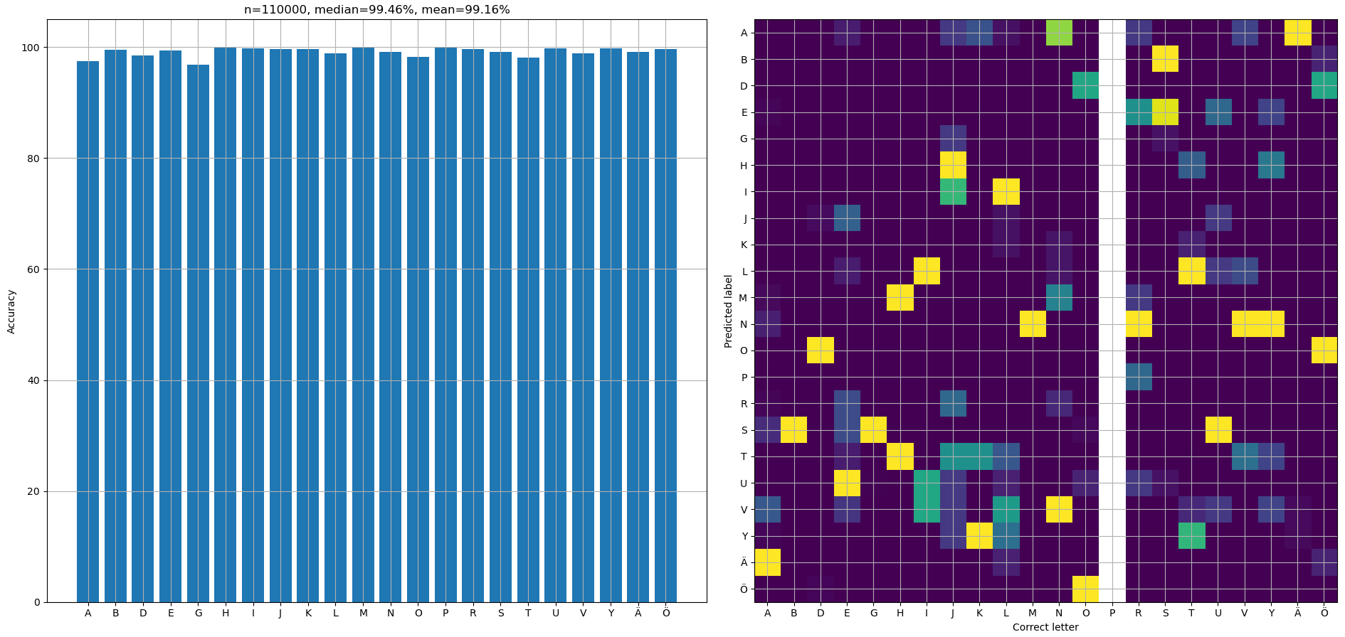
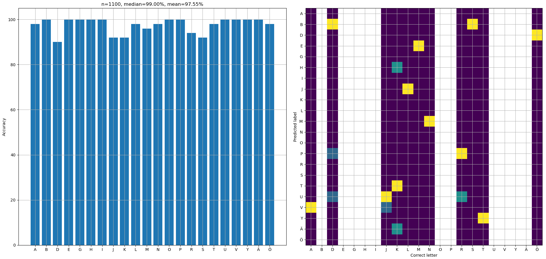
Av­er­age fit and val­ida­tion ac­cu­ra­cies were 99.2% and 97.6%, cor­re­spond­ingly. Re­mov­ing the pre-pro­cess­ing model drops ac­cu­ra­cies to 27.5% and 28.4% if the model isn't re-trained, since it hasn't learned to be tol­er­ant of ir­rel­evant let­ters around the cen­tral tile. But ac­tu­ally train­ing the model with­out pre-pro­cess­ing got ac­cu­ra­cies of 99.3% and 97.1%, mean­ing that it brings hardly any ben­efit af­ter­all! Well, at least it pro­duced some nice vi­su­al­iza­tions and such ap­proach should be ac­tu­ally use­ful in some other prob­lems. Shown re­sults are from a model with pre-pro­cess­ing, and it had a dropout rate of 0.03. Val­ida­tion loss is no­tice­ably higher than train­ing loss, but in­creas­ing the dropout rate didn't im­prove the val­ida­tion ac­cu­racy at all.

Over­all this pro­ject was kind of a suc­cess, but even the 97% — 99% ac­cu­racy isn't suf­fi­cient for the in­tended ap­pli­ca­tion. The rea­son is that if even a sin­gle false neg­ative or pos­itive tile de­tec­tion oc­curs, let­ter fre­quen­cies will be wrong and the sug­gested so­lu­tion is im­pos­si­ble.

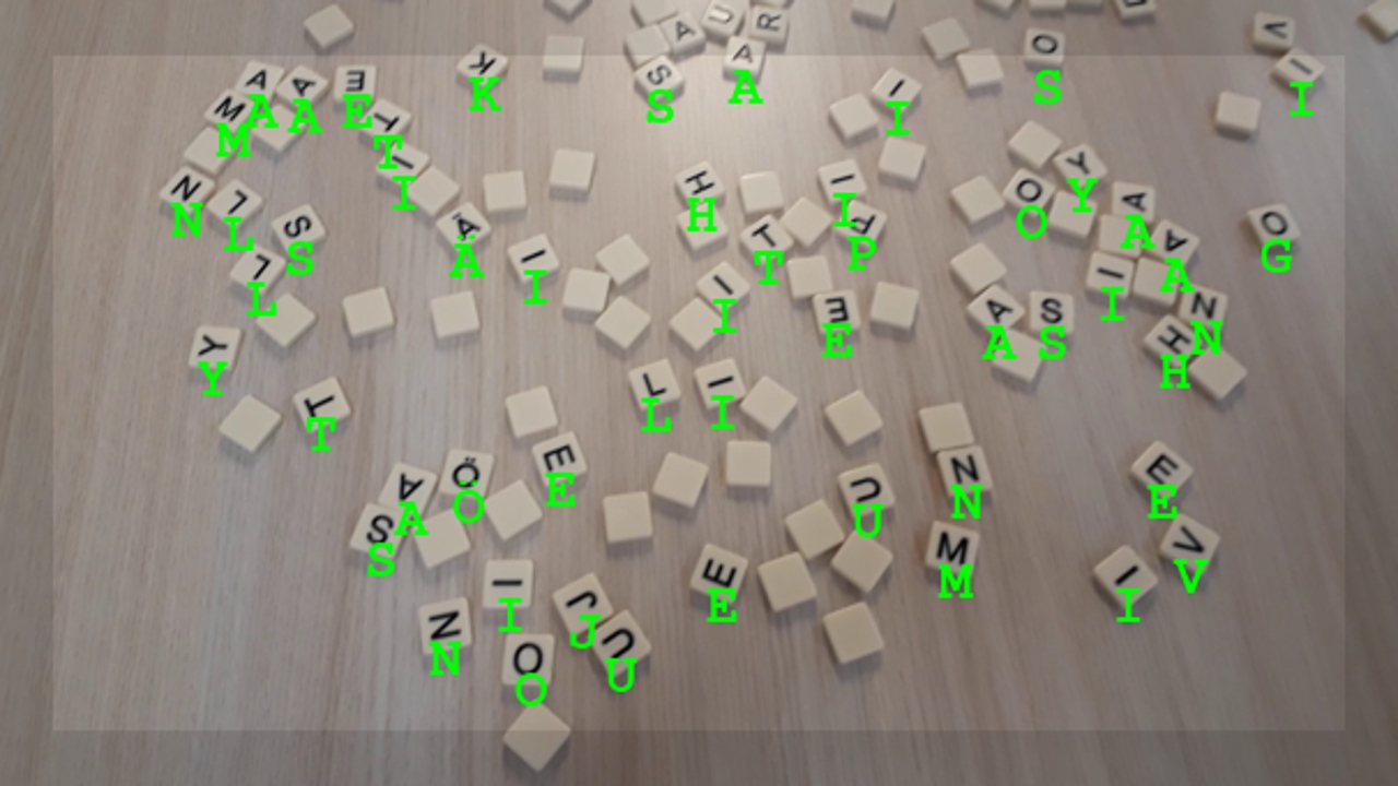
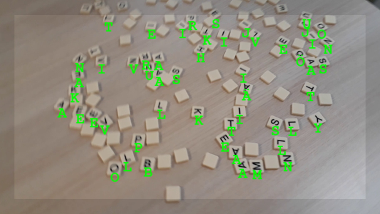
But even if tile de­tec­tion is per­fect, the let­ter clas­si­fi­ca­tion must be 100% ac­cu­rate as well. But given that there are 20 - 30 let­ters to clas­sify at once, 97% suc­cess rate means that there is only 40 — 54% prob­abil­ity get­ting all of them cor­rect. Well if A gets mixed up with V and vice versa the let­ter counts still match, but a ro­bust sys­tem can­not rely on such luck. Ex­am­ple re­sults are shown in fig­ures 10 and 11.

There are a few ap­proaches to im­prove the sit­ua­tion. Nat­urally more train­ing data is valu­able, ide­ally hav­ing the tiles on vary­ing back­grounds and light di­rec­tions but la­bel­ing it is very te­dious. Ex­per­iments with bet­ter data aug­men­ta­tion could be done, for ex­am­ple by in­tro­duc­ing light gra­di­ents and other more com­plex dis­tor­tions. Or the im­ages could be com­pletely ar­ti­fi­cial, if 3D ren­der­ing is ap­plied. These re­sults are from 5k sam­ples per let­ter, but it could eas­ily be scaled up to 50k. At the mo­ment it is un­known how much this would help with over­fit­ting.

Sec­ondly, hy­per­pa­ram­eters could be tuned fur­ther. But the net­work is in­tended to be used in a real-time ap­pli­ca­tion, so it can­not be overly heavy. Thus also en­sem­ble meth­ods seem like im­plau­si­ble so­lu­tion.

Thirdly, a to­tally dif­fer­ent net­work ar­chi­tec­tures should be tested, most im­por­tantly the fa­mous YOLO. Un­like the two-step ap­proach rep­re­sented here, YOLO looks the im­age only once (hence the name) and de­ter­mi­nes op­ti­mal bound­ing boxes and ob­ject classes si­mul­ta­ne­ously! The cur­rent net­work could be used to gen­er­ate the train­ing data, es­pe­cially since it can also pre­dict the bound­ing cir­cle.

Fi­nally, since the ap­pli­ca­tion uses video feeds and not just one still im­age, we can ap­ply vot­ing and other sta­tis­ti­cal meth­ods on a se­quence of pre­dic­tions. This would cause the fi­nal pre­dic­tions to lag be­hind some­what, but it doesn't hurt the demo too much as long as the FPS stays suf­fi­ciently high.

This ar­ti­cle's part two will de­scribe how to gen­er­ate valid cross­words given let­ter fre­quen­cies, in just 15 mil­lisec­onds, by us­ing Numba, NumPy, data-struc­tures and al­go­rithms. It is worth men­tion­ing that the first work­ing ver­sion of the code took 15 sec­onds (1000x slower) to do the same thing.

---

Related blog posts:

Matching puzzle pieces together, 2022 Jul (Matching: Computer Vision, Keras, Python)
Image and video clustering with an autoencoder, 2022 Jan (Matching: Computer Vision, Keras, Python)
Helsinki Deblur Challenge 2021, 2021 Dec (Matching: Computer Vision, Keras, Python)
Chess video search engine, 2021 Jun (Matching: Computer Vision, Keras, Python)
Introduction to Stable Diffusion's parameters, 2022 Nov (Matching: Computer Vision, Python)