
Since hearing the news of a faling Chinese rocket booster Long March 5B and being reminded that Earth's surface is about 70% ocean, I got interested on how the orbital parameters affect the odds of crashing to ocean vs. ground. I was nearly finished with the project when I realized that Earth is rotating under the satellite, thus invalidating all the results! This doesn't take orbits' eccentricity into account either, but I've heard that the athmospheric drag has a dendency of reducing it to zero as the orbit falls. Anyway, I found the various "straight" paths around the globe interesting and decided to publish these results anyway. In conclusion there are paths which spend only 9 % on top of land (including lakes) and 91% on top of ocean or up-to 57% on top of land and 43% on top of ocean.
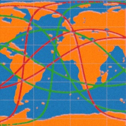
At first I started looking for a geographical dataset for Python. I wound an excellent article from towardsdatascience.com which introduced me to "ETOPO1 Global Relief Model" published by NOAA. It consists of a 21601 × 10801 grid (→ 223 million datapoints) of Earth's surfaces height in reference to the sea level (meaning lakes above the sea level as classified as dry land), having on average a measurement on every 1.5 × 1.5 km2 area. We don't need this kind of precision and can start by dropping 99% of the data, leaving us with 2.3 million samples and each covering on average an area of 15 × 15 km2. However the dataset is uniformy sampled in latitude & longitude coordinates, which means that poles are more densely sampled than the equator. This doesn't matter on some applications, but when calculating the average time spent on top of ocean it is important to have an unbiased sample. This is easily fixed by dropping out samples in proption to 1 - cos(lat). This drops about 36% of data, leaving us with 1.5 million samples and each representing an area of 19 × 19 km2.
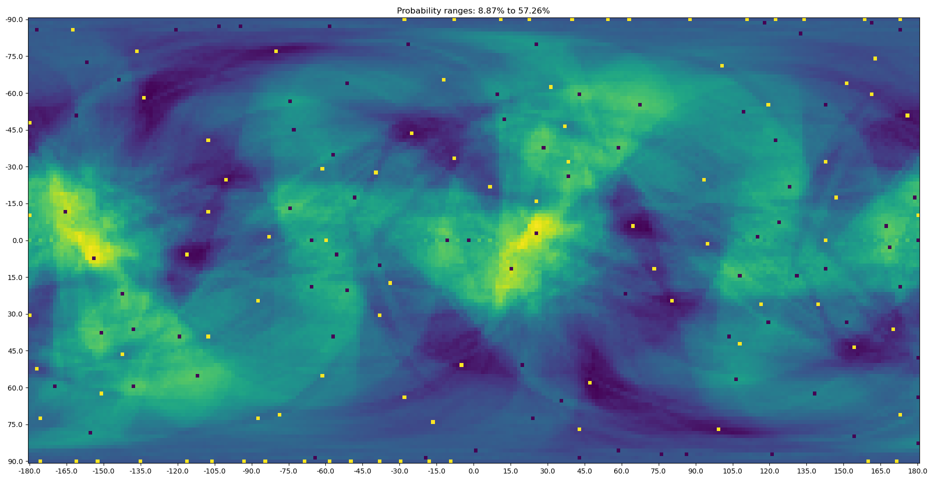
Once we have an uniform sample in lat & lon coordinates it is trivial to transform them to the unit sphere in 3D cartesian coordinates. A great circle is parameterized by a 3D unit vector, and it consists of points of which's coordinates dot product with the unit vector is zero. Naturally we must allow some tolerance to this, for example a \pm 100 km threshold corresponds to the dot product's absolute value being \le 100km / (2π * 6370km) → 0.00245. The easiest way of finding optimal great circles (minimizing or maximizing the dry land) is to brute-force the result on a search grid and finding local minima and maxima. The result of this is shown in Figure 1 (I learned only afterwards that this is called the Funk Transform). Again, an uniform sampling in lat & lon coordinates is not uniform in 3D space but it isn't as important here as it is in the underlying ocean vs, ground data. We just need to be mindful that the parameter space near the poles is over-sampled, and apply a secondary filter to ignore near duplicate great circles. The similarity is measured by the dot product of their unit vectors, and it approaches one (being the cosine of the angle between them) when the vectors point to a similar direction.
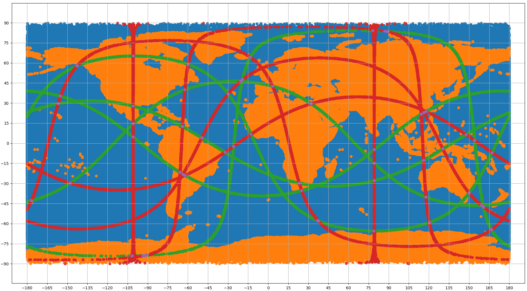
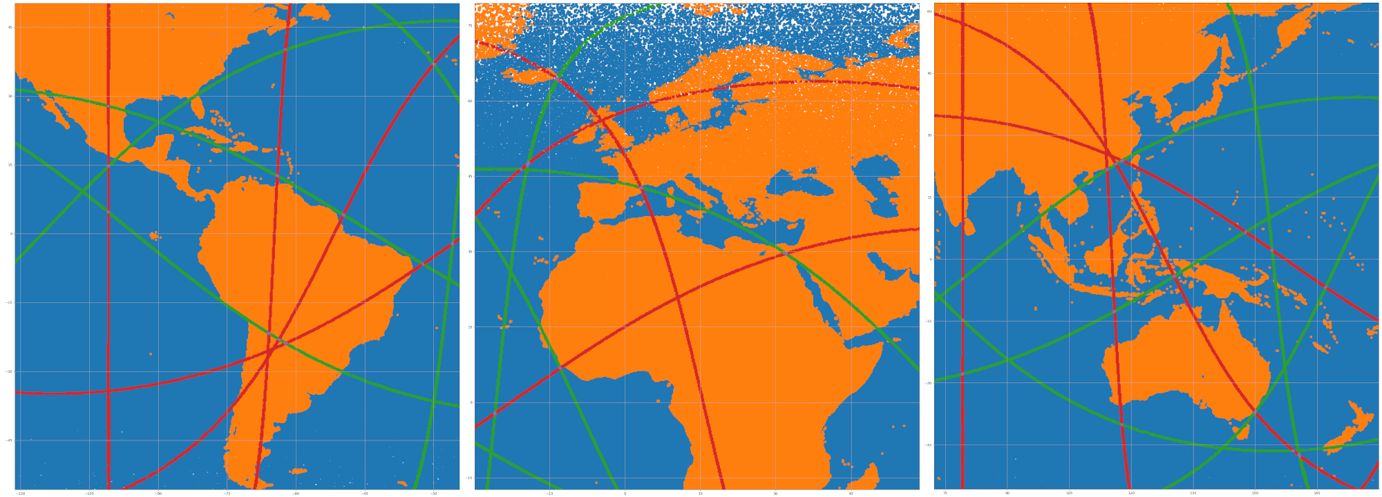
Once the filtering is done we can visualize most distinct paths on a map as shown in Fiugre 2. This doesn't use any fancy map projection, so polar regions are exaggerated in size. It is interesting how many of the oeacn-maximizing paths hug the coastal line. Some zoomed regions are shown in Figure 3, which also shows how polar regions are more sparsely sampled in lat & lon coordinates to make them uniform in the cartesian space.
Related blog posts:
|
|
|
|
|
|
|
|
|
|
