Niko's Project Corner

---

Youtube has a quite good search func­tion­al­ity based on video ti­tles, de­scrip­tions and maybe even sub­ti­tles but it doesn't go into ac­tual video con­tents and provide ac­cu­rate times­tamps for users' searches. An youtu­ber "Agad­ma­tor" has a very pop­ular chan­nel (1.1 mil­lion sub­scribers, 454 mil­lion video views at the time of writ­ing) which show­cases ma­jor chess games from past and re­cent tour­na­ments and on­line games. Here a search en­gine is in­tro­duced which an­alyzes the videos, rec­og­nizes chess pieces and builds a database of all of the po­si­tions on the board ready to be searched. It keeps track of the ex­act times­tamps of the videos in which the queried po­si­tion oc­curs so it is able to provide di­rect links to rel­evant videos.

I am a be­gin­ner on­line chess player my­self, hav­ing started in De­cem­ber 2020 at Chess.com (≈1200 rat­ing in 10 min rapid) thanks to the "ca­sual" PogChamps tour­na­ment. I had fol­lowed Agad­ma­tor for a long time be­fore this event, and de­cided to fi­nally put some moves on the board my­self. The search en­gine is hosted as a sin­gle-page-app at AWS S3, writ­ten in Clo­jure­Script (Reagent) but relying on pre-calculated data structure generated by Python and Keras.

The first step was down­load­ing all the videos form Youtube, which was very easy thanks to youtube-dl. You can get the list of video ids by youtube-dl -j --flat-playlist $URL and use youtube-dl -o "id_$ID.webm" -f $FOR­MAT "https://www.youtube.com/watch?v=$ID" to down­load them. It is note­wor­thy that $ID can start with a -, so it is good to prefix file names with something to avoid cli args confusion or make sure each call has -- at an appropriate place. File size can be minimized by using 720p video streams, having $FORMAT code either 136 or 247. Agadmator has been doing videos for a long time, and apparently Youtube has been changing codecs behind the scenes so one must chech that in which format each video exists. Also these videos do not contain audio, if you wish to include it you can download file formats 249, 251 or 140 of low-quality streams. Video and audio were then compressed further by ffmpeg and the video was reduced to 4 frames per second by a command like ffmpeg -nostats -loglevel error -hwaccel cuvid -i "$vid.v.webm" -c:v hevc_nvenc -rc vbr_hq -qmin:v 28 -qmax:v 30 -x265-params range=full -dst_range 1 -pix_fmtyuv420p -movflags faststart -an -r 4 -vf scale=1280:720 "$vid.mp4". Audio was compressed by ffmpeg -nostats -loglevel error -i "$vid.a.webm" -codec:a libmp3lame -af aresample=22000 -b:a 16k -ac 1 "$vid.mp3" and these are then merged into a single file via ffmpeg -nostats -loglevel error -i "$vid.mp4" -i "$vid.mp3" -c:v copy -c:a copy -y "../videos/$vid.mp4". In total about 700 hours of content was downloaded but it takes only 20 GB of disk space.

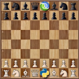
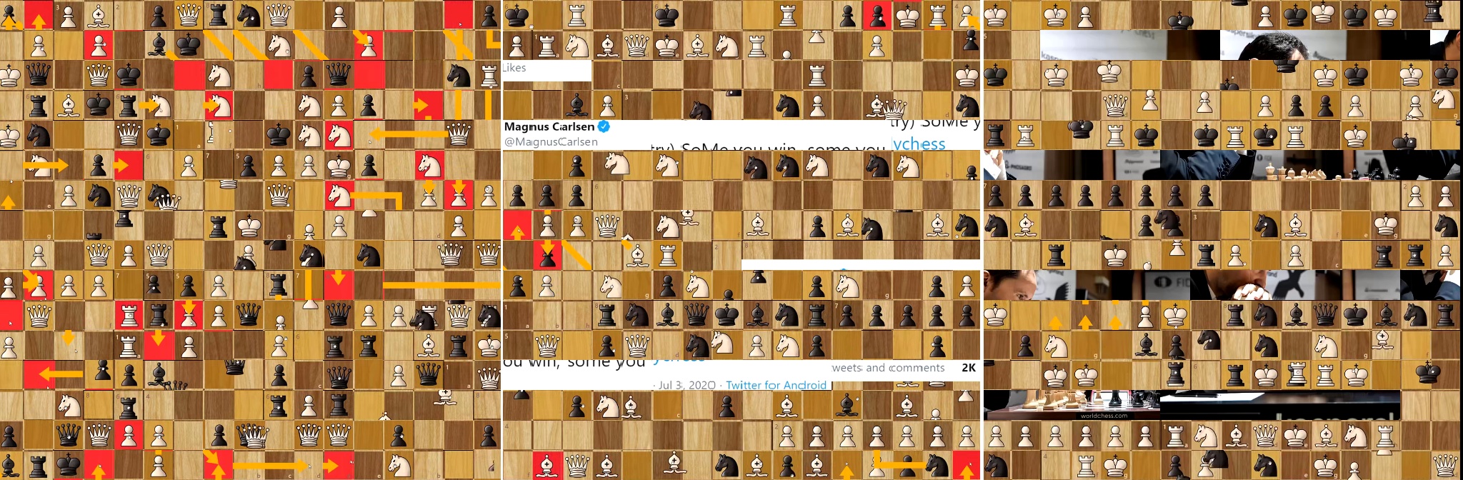
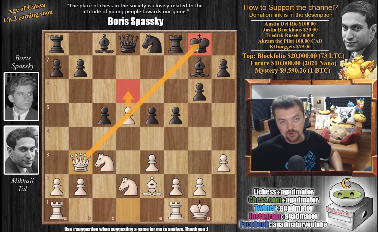
The first has­sle was to crop the chess board from the video, and this can­not be hard-coded since Agad­ma­tor has used two dif­fer­ent lay­outs in his videos (Fig­ure 1). Each video was clas­si­fied to the old and new for­mats based on the 10th frame of the video (at 4 fps), but ac­tu­ally re­cently he has been do­ing some in­tro­duc­tion at the be­gin­ning of the video which spoils this sim­ple logic. Luck­ily when in doubt we can guess that the video uses the new lay­out, or hard-code the class of the few prob­lem­atic ids. Also some videos aren't a typ­ical chess game anal­ysis at all and must be skipped.

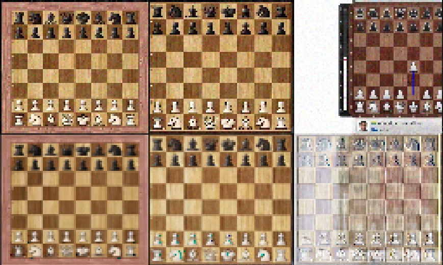
The video clas­si­fier was trained by grab­bing the 10th frame, re­siz­ing it to a small 160 × 90 res­olu­tion and crop­ping a 77 × 86 area from it. There is also some noise added to this crop­ping pro­cess, to make the model more re­silient of mi­nor de­vi­ations of Agad­ma­tor's lay­out be­tween videos. These cropped re­gions were then used to train an 1D au­toen­coder. Ex­am­ple crops and their au­toen­coder out­puts are shown in Fig­ure 2.

The au­toen­coder has a quite ba­sic ar­chi­tec­ture: a se­quence of con­vo­lu­tions and pool­ing lay­ers bring the im­age down to a smaller size, fi­nal few dense lay­ers crush it into one or two di­men­sions, and a stack of dense lay­ers pro­gres­sively bring it back to the orig­inal res­olu­tion. The em­bed­ding layer has tanh ac­ti­va­tion which lim­its the range be­tween -1 and 1, and the fi­nal layer has sig­moid which lim­its the RGB out­put be­tween 0 and 1. I have found that relu ac­ti­va­tion works well on con­vo­lu­tional lay­ers, but elu has more "flex­ibil­ity" on re­gres­sion-type roles at dense lay­ers. Ac­tu­ally de­pend­ing on the mag­ni­tude of the in­put sig­nal and the layer's weights it can smoothly "in­ter­po­late" be­tween lin­ear and relu-like ac­ti­va­tion.

This ar­chi­tec­ture wasn't op­ti­mized that much, since it needs only to be good enough for this pur­pose. (Sorry the blog is lack­ing syn­tax high­light for non-PHP con­tent. The PDF ver­sion is pret­tier, and I must re­mind you that it is gen­er­ated di­rectly by L^aT_eX.)

• enc_dim = 1
• enc = Dense(enc_dim, activation='tanh')
• model = Sequential([
• Input(X.shape[1:]),
• Conv2D(16, 3, activation='relu'), BN(), AveragePooling2D(2),
• Conv2D(32, 3, activation='relu'), BN(), AveragePooling2D(2),
• Conv2D(64, 3, activation='relu'), BN(), AveragePooling2D(2),
• Conv2D(64, 3, activation='relu'), BN(),
• Flatten(),
• Dense(64, activation='elu'), BN(),
• Dense(32, activation='elu'), BN(),
• Dense(8, activation='elu'), BN(),
• enc,
• Dense(8, activation='elu'), BN(),
• Dense(32, activation='elu'), BN(),
• Dense(64, activation='elu'), BN(),
• Dense(256, activation='elu'), BN(),
• Dense(np.prod(X.shape[1:]), activation='sigmoid'),
• Reshape(X.shape[1:])
• ])

Al­though we are work­ing on a quite low res­olu­tion, the model has 5.3 mil­lion pa­ram­eters. This is mainly due to the last dense layer which ex­pands the rep­re­sen­ta­tion from 256 to 77 × 86 × 3 = 19866 di­men­sions.

• _________________________________________________________________
• Layer (type) Output Shape Param #
• =================================================================
• conv2d_16 (Conv2D) (None, 75, 84, 16) 448
• batch_normalization_44 (Batc (None, 75, 84, 16) 64
• average_pooling2d_12 (Averag (None, 37, 42, 16) 0
• conv2d_17 (Conv2D) (None, 35, 40, 32) 4640
• batch_normalization_45 (Batc (None, 35, 40, 32) 128
• average_pooling2d_13 (Averag (None, 17, 20, 32) 0
• conv2d_18 (Conv2D) (None, 15, 18, 64) 18496
• batch_normalization_46 (Batc (None, 15, 18, 64) 256
• average_pooling2d_14 (Averag (None, 7, 9, 64) 0
• conv2d_19 (Conv2D) (None, 5, 7, 64) 36928
• batch_normalization_47 (Batc (None, 5, 7, 64) 256
• flatten_4 (Flatten) (None, 2240) 0
• dense_37 (Dense) (None, 64) 143424
• batch_normalization_48 (Batc (None, 64) 256
• dense_38 (Dense) (None, 32) 2080
• batch_normalization_49 (Batc (None, 32) 128
• dense_39 (Dense) (None, 8) 264
• batch_normalization_50 (Batc (None, 8) 32
• dense_36 (Dense) (None, 1) 9
• dense_40 (Dense) (None, 8) 16
• batch_normalization_51 (Batc (None, 8) 32
• dense_41 (Dense) (None, 32) 288
• batch_normalization_52 (Batc (None, 32) 128
• dense_42 (Dense) (None, 64) 2112
• batch_normalization_53 (Batc (None, 64) 256
• dense_43 (Dense) (None, 256) 16640
• batch_normalization_54 (Batc (None, 256) 1024
• dense_44 (Dense) (None, 19866) 5105562
• reshape_4 (Reshape) (None, 77, 86, 3) 0
• =================================================================
• Total params: 5,333,467
• Trainable params: 5,332,187
• Non-trainable params: 1,280

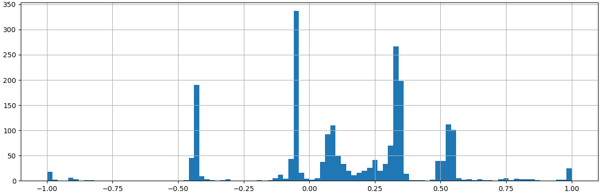
The en­coder model is con­structed sim­ply by enc_model = Model(model.in­put, enc.out­put). The en­coder puts each im­age type into a very dis­tinct value range, as can be seen at fig­ures 3 and 4. Ac­tu­ally in ad­di­tion to the in­put's en­coded value, whether it is an out­lier can be also de­tected from the rep­re­sen­ta­tion er­ror be­tween the in­put and out­put im­age but this was not im­ple­mented. Due to ran­dom ini­tial­iza­tion the net­work con­verges al­ways to a dif­fer­ent rep­re­sen­ta­tion for old and new types of boards. Any­way, in this case "bright" out­lier in­puts are in the range of -1 to -0.5, -0.5 to -0.4 cor­re­spond to the old lay­out, -0.2 all the way to 0.7 are new lay­outs and from 0.7 on­wards they seem to be darker out­liers.

Once this is done all rel­evant videos can be cropped and re­sized into a stan­dard res­olu­tion. The next step is to iden­tify the pieces (and pawns) on the board. This isn't as triv­ial as it might sound (I in­deed ex­pected this to be easy!), be­cause there are all kinds of graph­ics on the board and pieces move over each other. A rep­re­sen­ta­tive sam­ple of pieces on the board (and empty squares) was col­lected at an res­olu­tion of 42 × 42 each. This was done by go­ing through videos' frames and first drop­ping near-dub­pli­cate frames.

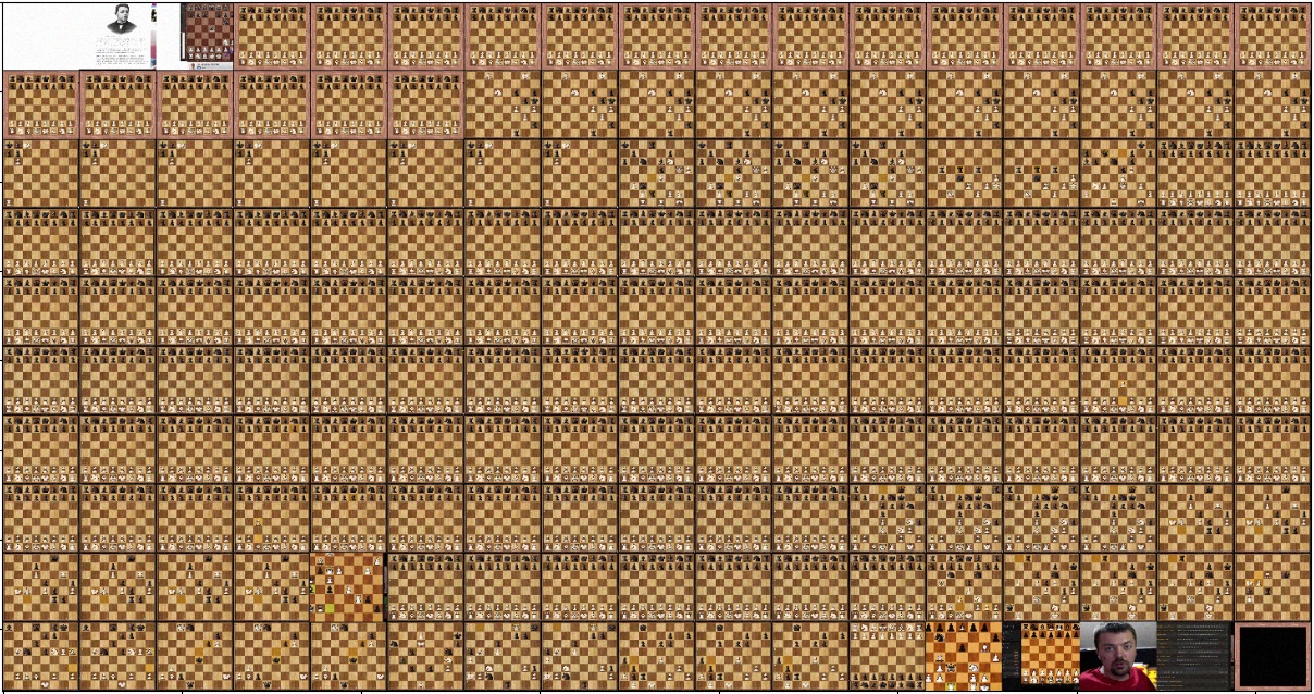
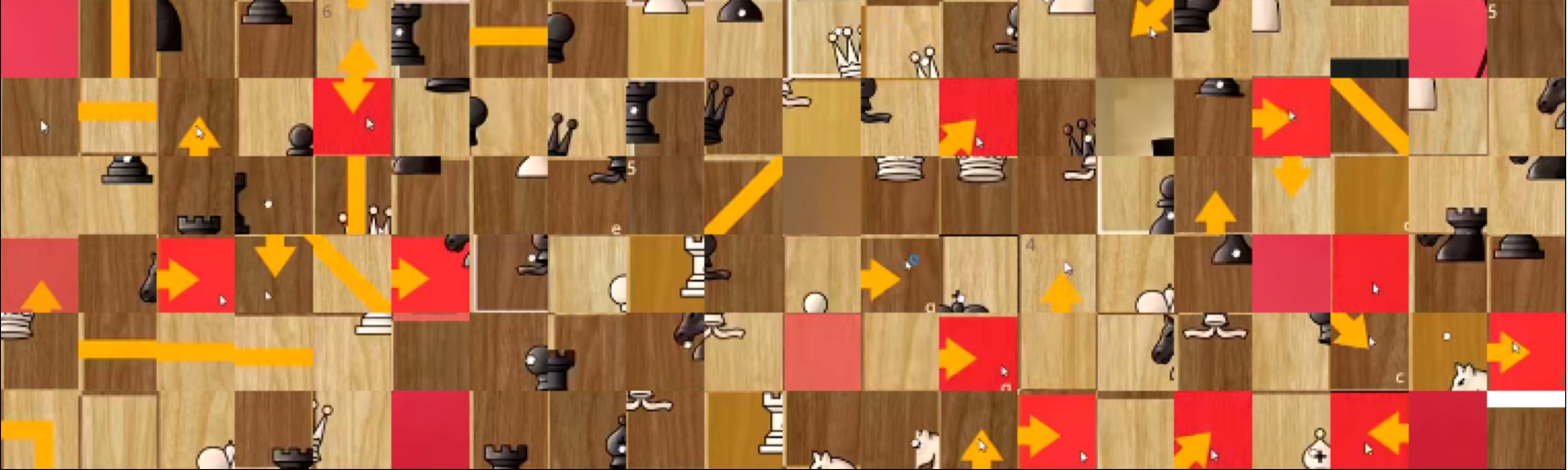
A buffer of 256 pieces was kept, and a new can­di­date piece was not added to the buffer if it was too sim­ilar to an al­ready ex­ist­ing one. This en­sures that the col­lec­tion doesn't have too much re­dun­dant sam­ples, which is es­pe­cially im­por­tant in this case since the pieces do not move on the board most of the time. This re­sults in 204 stored buffers, each hav­ing 256 crops so in to­tal there were 52k crops stored. Three buffers are shown in Fig­ure 5.

Many crops are "pol­luted" by hav­ing a red back­ground, hav­ing a yel­low ar­row go­ing across it or both. These are a very use­ful fea­tures of the chess board UI, used to high­light crit­ical squares, moves and piece pro­tec­tions. These make more sense in the con­text of a com­plete board, as seen in Fig­ure 6.

This col­lec­tion of un­la­belled data wasn't much use for the pur­pose of iden­ti­fy­ing pieces on the board. But man­ual la­bel­ing is very te­dious, so an ini­tial batch of dis­tinct im­ages was ex­ported by run­ning them through a new au­toen­coder (not en­cod­ing full chess boards, only in­di­vid­ual cropped squares) and iden­ti­fy­ing a few hun­dred dis­tinct im­ages. These are then la­beled man­ually and are run through the first su­per­vised neu­ral net­work. Since we have very lit­tle data, the first net­work has to be quite sim­ple to avoid over­fit­ting. Of course we can use some data aug­men­ta­tion in terms of ran­dom trans­la­tion, zoom­ing and ro­ta­tion but these do not cor­re­spond well to the kind of ob­struc­tions we have in the real dataset. All ver­sions of the net­work had the tra­di­tional "con­vo­lu­tion → dense → soft­max" ar­chi­tec­ture

So the ini­tial dataset is used to train a net­work, and it is used to do fore­casts. Since the last ac­ti­va­tion layer is soft­max, its out­puts kind of cor­re­spond to class prob­abil­ities. And we can this iden­tify the in­puts for which the net­work was most un­sure that to which class it be­longs to. These sam­plex are then ex­ported, man­ually la­belled and this pro­cess is iter­rated un­til the val­ida­tion er­ror is sat­is­fac­tory or the man­ual la­borer is ex­hausted. In to­tal 4200 im­ages were clas­si­fied. The dataset has a quite strong class im­palance, 28.4% of them is "par­tial" but only 2.1% are of "white_king" since those were the most dif­fi­cult and eas­iest classes. It would be in­ter­est­ing to re-visit this with a semisu­per­vised learn­ing method, but this will do for now. Here is a rea­son­able net­work ar­chi­tec­ture:

• dim, kernel, d, rot, zoom = 10, 9, 0.1, 10 / 360, 0.1
• model = Sequential([
• Input(X.shape[1:]),
• preprocessing.RandomRotation(rot),
• preprocessing.RandomZoom(zoom),
• Conv2D(dim, kernel, activation='relu'), D(d), BN(),
• Conv2D(dim, kernel, activation='relu'), MaxPooling2D(2), D(d), BN(),
• Conv2D(dim, kernel, activation='relu'), BN(),
• Flatten(),
• Dense(16, activation='elu'), BN(),
• Dense(n_cls, activation='softmax')
• ])

Model's sum­mary was the fol­low­ing:

• _________________________________________________________________
• Layer (type) Output Shape Param #
• =================================================================
• random_rotation_2 (RandomRot (None, 38, 38, 3) 0
• random_zoom_2 (RandomZoom) (None, 38, 38, 3) 0
• conv2d_150 (Conv2D) (None, 30, 30, 10) 2440
• dropout_4 (Dropout) (None, 30, 30, 10) 0
• batch_normalization_398 (Bat (None, 30, 30, 10) 40
• conv2d_151 (Conv2D) (None, 22, 22, 10) 8110
• max_pooling2d_2 (MaxPooling2 (None, 11, 11, 10) 0
• dropout_5 (Dropout) (None, 11, 11, 10) 0
• batch_normalization_399 (Bat (None, 11, 11, 10) 40
• conv2d_152 (Conv2D) (None, 3, 3, 10) 8110
• batch_normalization_400 (Bat (None, 3, 3, 10) 40
• flatten_38 (Flatten) (None, 90) 0
• dense_234 (Dense) (None, 16) 1456
• batch_normalization_401 (Bat (None, 16) 64
• dense_235 (Dense) (None, 15) 255
• =================================================================
• Total params: 20,555
• Trainable params: 20,463
• Non-trainable params: 92

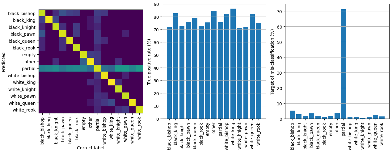
Even­tu­ally the val­ida­tion ac­cu­racy was about 85%, but this isn't as bad as it sounds. An ex­tra test was run, in which only 50% of data was used for train­ing and the other 50% for val­ida­tion. Fore­cast ac­cu­racy re­sults of the val­ida­tion set are shown in Fig­ure 7. As ex­pected the most dif­fi­cult class to pre­dict was the "par­tial" class, see Fig­ure 8 for ex­am­ples. Ba­si­cally they have two over­lap­pign pieces, which oc­curs when a piece is be­ing cap­tured. It is hard to set a thresh­old when the im­age should be clas­si­fied as two dis­tinct pieces or just one dom­inant one. How­ever this dis­tinc­tion isn't im­por­tant for this pro­ject's main pur­pose, since the square will be cor­rectly clas­si­fied once cap­ture is 100% done and the sit­ua­tion is sta­ble. An other tricky one is the "empty" class, when a piece is be­ing moved to the square. In this ex­per­iment the pre­ci­sion (per­cent­age of cor­rectly la­belled classes, or the di­ag­onal of the con­fu­sion ma­trix) was re­spectable 70 - 90%.

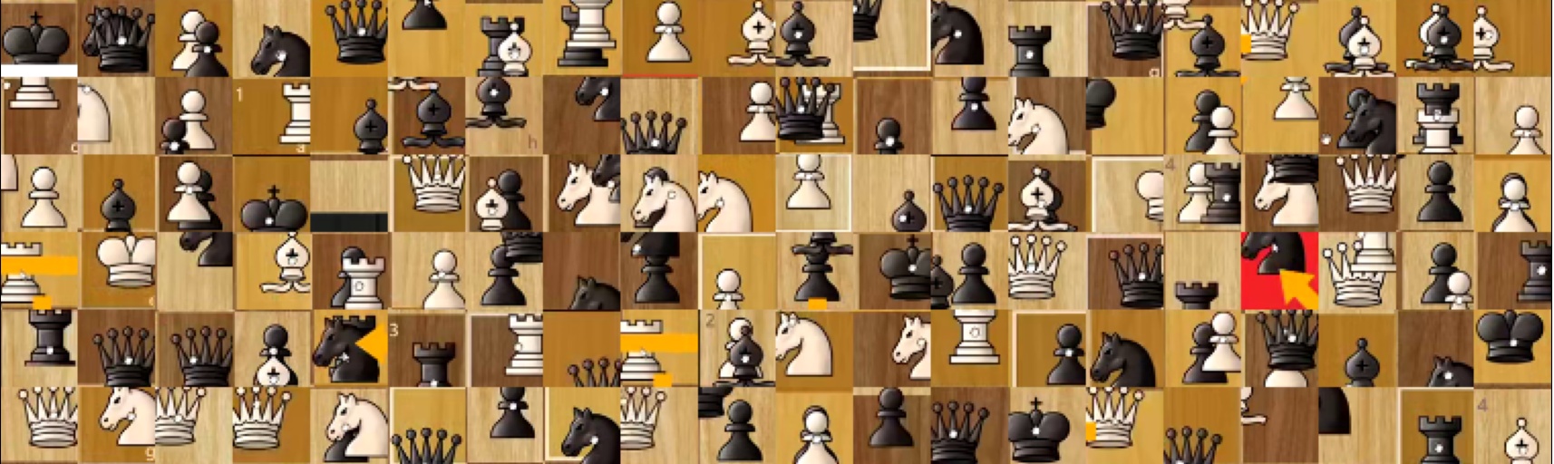
Empty squares aren't triv­ial ei­ther, be­cause when a piece is be­ing moved to it there comes a point when the cor­rect clas­si­fi­caiton is "par­tial". Sev­eral ex­am­ples are shown in Fig­ure 9. Again the dis­tinc­tion be­tween the two isn't cru­cial in the end, since it will be cor­rectly la­beled once the piece is dropped on the board and the sit­ua­tion is sta­ble.

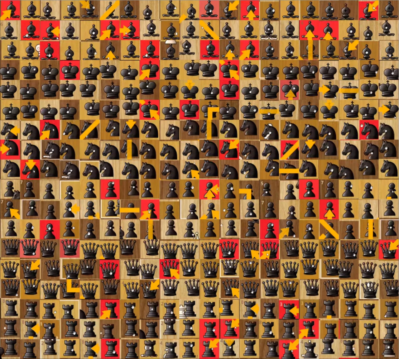
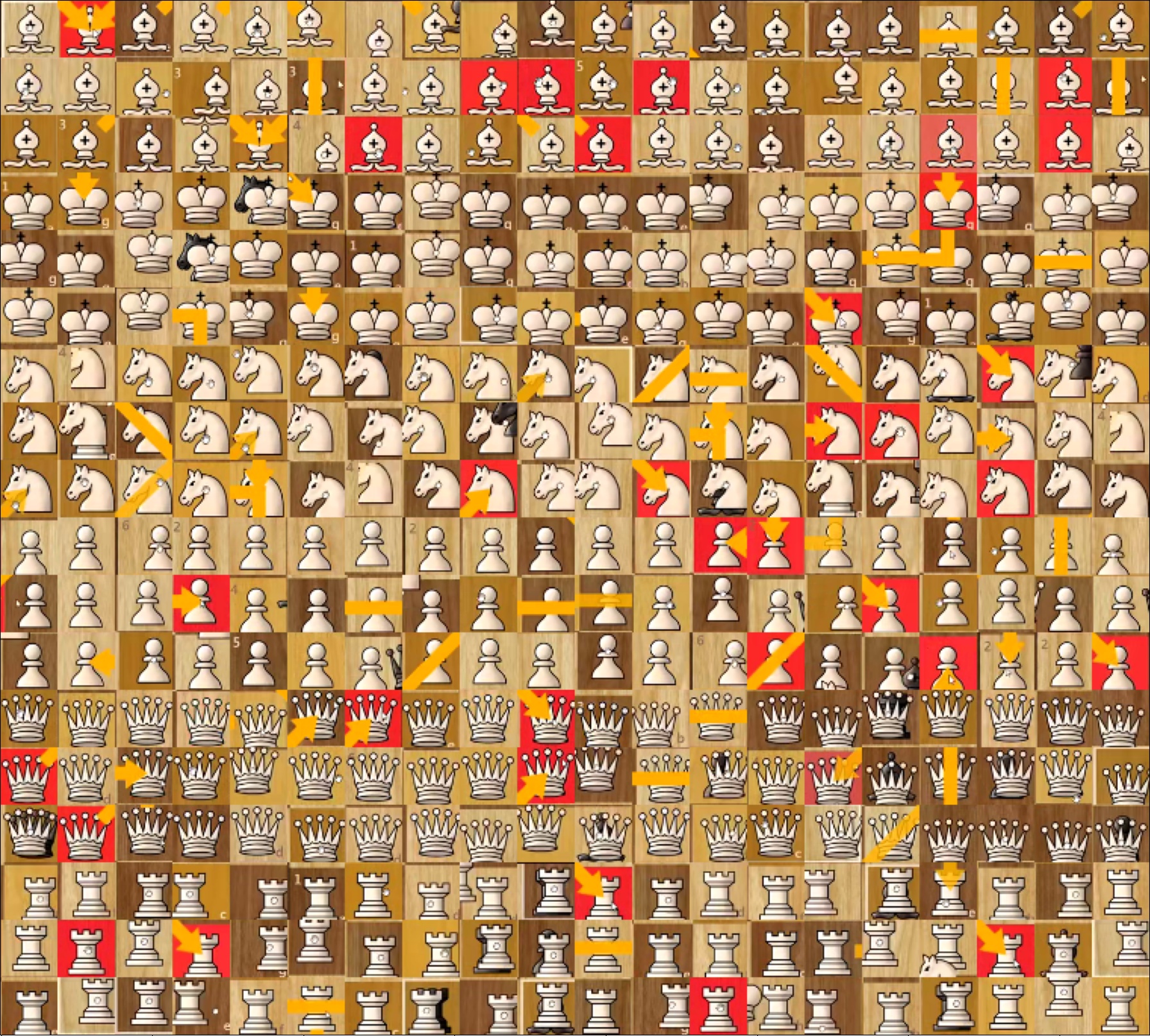
Ex­am­ples of black chess pieces (and pawns) are shown in Fig­ure 10. It shows a va­ri­ety of piece's po­si­tions within the crop, ob­struc­tions by yel­low ar­rows, vary­ing back­grounds etc. Ex­am­ples of white pieces (and pawns) are shown in Fig­ure 11.

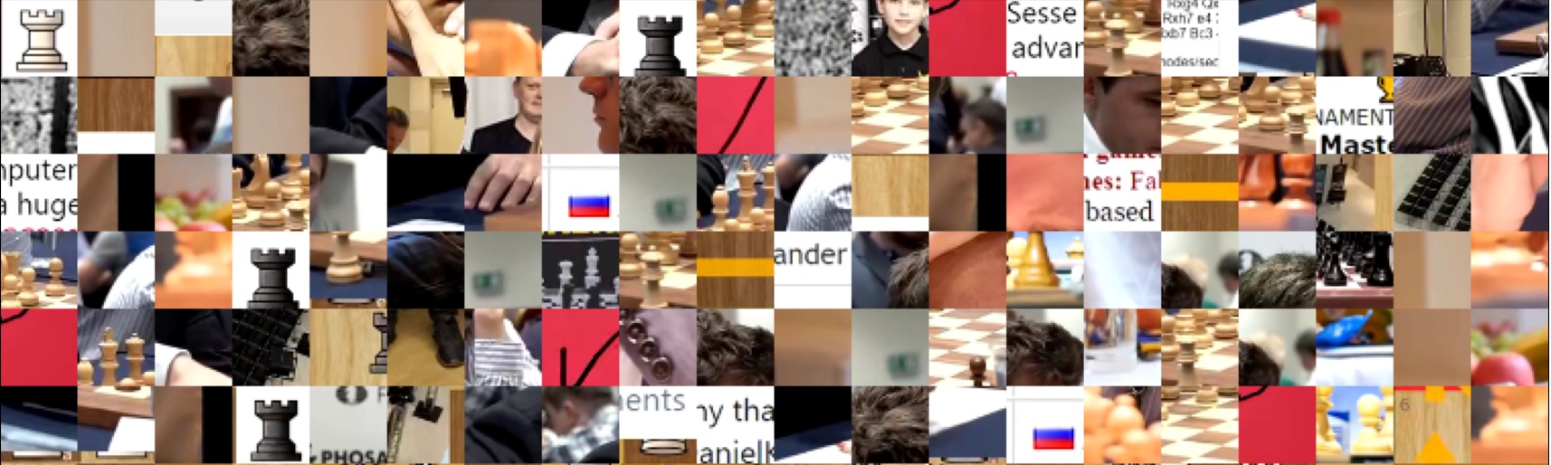
The fi­nal odd class is the "other", sam­ples are shown in Fig­ure 12. Ba­si­cally it con­sists of anyt­ing not re­lated to the chess board, which oc­cur when Agad­ma­tor is show­ing other con­tent re­lated to the game he is de­scrib­ing. The top left ex­am­ple is an ex­cep­tion, it is a white rook on a com­pletely white back­ground. This acu­tally hap­pens on the board when a white pawn is be­ing pro­moted, and there is a menu to choose which piece you want. I had these as a sep­arate la­bel in the train­ing data but de­cided to com­bine them with "other" since the dis­tinc­tion isn't im­por­tant in this case.

Once this net­work is suc­cess­fully trained as well we are done! We have a pipeline which down­loads a video from Youtube, com­presses it to lower bi­trate and FPS, de­tect whether it is the new or old lay­out and crop it ac­cord­ingly and iden­tify all pieces (and empty squares) on the board. This is ac­tu­ally just 300 - 400 lines of code, but nat­urally this in­volved lots of hy­per-pa­ram­eter tun­ing and other prob­lem solv­ing. The video is pro­cessed by load­ing cropped frames in batches and pass­ing through the clas­si­fier net­work. Ac­tu­ally the pre­vi­ously de­scribed model pro­cesses only one 38 × 38 × 3 in­put im­age, but as we know the chess board con­sists of a 8 × 8 grid of these. Luck­ily it is triv­ial to build a "com­bined" net­work which takes a 304 × 304 × 3 in­put, crops it into 64 38 × 38 × 3 squares and passes them to the sin­gle-square model. The re­sult is then con­cate­nated into a sin­gle 15 × 8 × 8 out­put, cor­re­spond­ing a class prob­abil­ity for each square out of the 15 classes (6 white pieces, 6 black pieces, "empty", "par­tial" and "other").

So a batch of 32 frames re­sults in an out­put of size 32 × 15 × 8 × 8, to which we can ap­ply numpy.argmax to find the most likely clas­si­fi­ca­tion for each of the 32 × 8 × 8 squares. Once the full video is pro­cessed we have a Numpy ar­ray of shape n × 8 × 8, each item hav­ing a value be­tween 0 and 14. (since there are 15 classes) We know that to which times­tamp each sam­ple cor­re­sponds to sim­ply based on the con­stant FPS of the video. A con­sec­utive "runs" of these classes are then stored into a JSON file in a time­line-like data struc­ture. This is the small­est data file from a video ti­tled Merry Christ­mas Chess Puz­zle to Brighten Your Day:

• {
• "id": "6qZDMNl8yXA",
• "title": "Merry Christmas Chess Puzzle to Brighten Your Day :)",
• "black_bishop": {
• "b8": [[0.00, 1.85], [2.23, 2.55]],
• "f4": [[2.08, 2.10]]
• },
• "black_king": {
• "a8": [[0.00, 2.55]]
• },
• "black_pawn": {
• "a6": [[2.42, 2.55]],
• "a7": [[0.00, 2.08], [2.27, 2.55]],
• "b7": [[0.00, 2.27], [2.29, 2.31]]
• },
• "white_king": {
• "c8": [[0.00, 2.55]]
• },
• "white_pawn": {
• "b6": [[0.00, 2.31]],
• "b7": [[2.45, 2.55]]
• },
• "white_rook": {
• "a1": [[2.24, 2.29]],
• "a6": [[1.85, 2.08], [2.31, 2.41]],
• "a7": [[2.10, 2.23]]
• }
• }

Each num­ber rep­re­sents a times­tamp in min­utes, for ex­am­ple we can see that the black king spent the en­tire game at a8 but a black bishop spent only (2.10 - 2.08) * 60 = 1.2 sec­onds in f4. (Ac­tu­ally if you check the video it stays there from 2:04 to 2:12, I should do some de­bug­ging to see what went wrong here. At least it wasn't mis­clas­si­fied as any other piece be­tween 2.10 - 2.20 (2:06 - 2:12).)

The ap­pli­ca­tion doesn't use that for­mat though, in­stead it uses a few tricks to com­press the data by about 50%. Firstly we don't need to store the times­tamps as lists of two-item lists, in­stead we can flat­ten the struc­ture and use Clo­jure's par­ti­tion to split it back into chunks. Sec­ond, we can store just each se­quence's first item as-is, and for the rest we store the in­ter­val be­tween the val­ues. Es­pe­cially on longer videos this leads to small num­bers (less than 10), for ex­am­ple [[3, 5], [7, 11], [12, 13], [19, 22]] is flattened to [3, 5, 7, 11, 12, 13, 19, 22] and calculating deltas leaves us with [3, 2, 2, 4, 1, 1, 9, 3]. The third optimization is not to work with floating point values with decimals, rather multiply each (delta) timestamp by 100 and store it as a fixed-point integer. This way we don't need to store the decimal separator either. In the shown JSON the numbers aren't stored in an array, rather it is a string where values are separated by spaces. This allows us to omit values of zero, which wouldn't be a valid JSON syntax. But actually I forgot to implement this optimization, so the used data structure is as follows:

• {
• "id": "6qZDMNl8yXA",
• "title": "Merry Christmas Chess Puzzle to Brighten Your Day :)",
• "black_bishop": {
• "b8": "0 185 37 31",
• "f4": "208 2"
• },
• "black_king": {
• "a8": "0 254"
• },
• "black_pawn": {
• "a6": "242 12",
• "a7": "0 208 18 27",
• "b7": "0 227 2 2"
• },
• "white_king": {
• "c8": "0 254"
• },
• "white_pawn": {
• "b6": "0 231",
• "b7": "245 9"
• },
• "white_rook": {
• "a1": "224 4",
• "a6": "185 23 23 10",
• "a7": "210 12"
• }
• }

In­dex­ing each video into this for­mat is quite speedy, run­ning at about 15 min­utes of video (3.6k frames since it was stored in 4 FPS) in one min­ute, or 1 hour in 4 min­utes. Pro­cess­ing all of them still takes a sig­nif­icant amount of time since there is about 500 hours of rel­evant videos (200 hours are from other long-for­mat streams), about 33 hours. Luck­ily the pro­cess can be run in par­al­lel, to push the to­tal time down to 10 - 15 hours. Nat­urally the full in­dex­ing has to be run only when the piece de­tec­tion net­work has been up­dated. A new video can be in­dexed "in­cre­men­tally", and just a new com­bined JS file has to be con­cate­nated and up­loaded to S3.

Speak­ing of which, the full dataset is avail­able here (at the mo­ment about 5.7 MB of JS), and it is loaded to the Clo­jure­Script ap­pli­ca­tion upon start-up. The ap­pli­ca­tion it­self is fairly sim­ple, the only in­ter­est­ing bit was im­ple­ment­ing the search al­go­rithm of this datased based on a (par­tial) sit­ua­tion on the board. Cur­rently it only searches match­ing pieces at given lo­ca­tions, you can­not query for a speci­fic square to be empty. Al­though this would be easy to im­plmenet post-hoc. At least for now this pro­ject isn't avail­able at GitHub, mainly due to how dirty the video pro­cess­ing and model train­ing pipeli­nes are. The Clo­jure­Script por­tion is only about 200 lines of code.

When the ap­pli­ca­tion starts and Clo­jure­Script gets eval­uated, it first con­verts the "global" videos ob­ject into a Clo­jure data struc­ture (and un­dos all the com­pres­sion steps which were de­scribed ear­lier) by uti­liz­ing the goog.ob­ject from Google's Clo­sure li­brary. Here are a few util­itiy func­tions (sorry my blog en­gine does not rep­re­sent Clo­jure code prop­erly since it gets stuff mixed with L^aT_eX rules such as % be­ing a com­ment, check the PDF for com­plete source code):

• (defn obj->clj [obj]
• (case (goog/typeOf obj)
• "array"
• (mapv obj->clj obj)
• "object"
• (-> (fn [result key]
• (let [v (goog.object/get obj key)]
• (if (= "function" (goog/typeOf v))
• result
• (assoc result key (obj->clj v)))))
• (reduce { } (.getKeys ^js/object goog/object obj)))
• obj))
• (defn str->floats [s]
• (let [result
• (->> (clojure.string/split s #" ")
• (map #(->
• js/parseInt
• (* 0.01))))]
• (assert (not-any? js/isNaN result) s)
• result))

The code which con­verts the list of "video" ob­jects (hash-maps) into a sin­gle large hash-map (where keys are video ids) is a bit deeply nested, but here is the main part of it:

• (fn [video]
• [(video "id")
• {:title (video "title")
• :moves (-> video
• (dissoc "id" "title")
• (->> (map (fn [[piece-str coord->ts]]
• [(->> (clojure.string/split piece-str #"_")
• (mapv keyword))
• (zipmap (->> coord->ts keys (map keyword))
• (->> coord->ts
• vals
• (mapv
• #(->>
• str->floats
• (reductions +)
• (partition 2)))))]))
• (into { })))}])

And this is the larger con­text:

• (defonce videos
• (let [t0 (.now js/Date)
• result
• (->> js/videos
• (map obj->clj)
• (map (fn [video] ...))
• (into { }))]
• (swap! init-times assoc 'videos (- (.now js/Date) t0))
• result))

Clo­jure­Script's de­fonce makes it very pleas­ant to work with state­ful data with pure func­tions. You can have your func­tions hot-reloaded in an in­stant with­out los­ing you ap­pli­ca­tion's state, it feels like magic! De­com­press­ing the data takes about 2.2 sec­onds. Us­ing the same video as an ex­am­ple, its Clo­jure data struc­ture looks like this:

• ; (videos "6qZDMNl8yXA")
• {:title "Merry Christmas Chess Puzzle to Brighten Your Day :)",
• :moves
• {[:black :king] {:a8 ((0 2.5))},
• [:black :pawn] {:a6 ((2.41 2.49)), :a7 ((0 2.08) (2.26 2.49)),
• :b7 ((0 2.25) (2.26 2.3))},
• [:white :rook] {:a1 ((2.25 2.27)), :a6 ((1.85 2.08) (2.31 2.41)), :a7 ((2.1 2.22))},
• [:white :queen] { },
• [:white :king] {:c8 ((0 2.5))},
• [:white :pawn] {:b6 ((0 2.31)), :b7 ((2.45 2.49))},
• [:black :rook] { },
• [:black :queen] { },
• [:black :bishop] {:b8 ((0 1.85) (2.22 2.49)), :f4 ((2.08 2.1))},
• [:white :knight] { },
• [:white :bishop] { },
• [:black :knight] { }}}

An other im­por­tant data struc­ture is state->ids which maps ev­ery ex­ist­ing square co­or­di­nate and chess piece to a set of video ids which have that sit­ua­tion hap­pen­ing at some point in game. Build­ing this takes about 1.8 sec­onds.

• (defonce state->ids
• (let [t0 (.now js/Date)
• result
• (->> videos
• (map (fn [[id video]]
• (->> (for [[piece transitions] (:moves video)
• coord (keys transitions)]
• [[coord piece] [id]])
• (into { }))))
• (apply merge-with into))
• result (zipmap (->> result keys)
• (->> result vals (map set)))]
• (swap! init-times assoc 'state->ids (- (.now js/Date) t0))
• result))

The list of 20 rarest pieces & po­si­tions looks like this (ac­tu­ally those pawn re­sults from ranks 1 & 8 are bugs, most likely mis-iden­ti­fied bish­ops!):

• ; (->> state->ids (sort-by (comp count val)) (take 20))
• ([[:b8 [:white :pawn]] #{"eDUCzsu0ZIU"}]
• [[:h1 [:white :pawn]] #{"vaJ2wj3azyw"}]
• [[:b1 [:black :pawn]] #{"Undasf0tKYQ"}]
• [[:h8 [:black :pawn]] #{"BcVu_ZM8R5A"}]
• [[:h8 [:white :pawn]] #{"1DZDoKElZFo"}]
• [[:c1 [:black :pawn]] #{"Undasf0tKYQ"}]
• [[:c8 [:black :pawn]] #{"Undasf0tKYQ"}]
• [[:a1 [:black :king]] #{"w2BWmSBog_0" "quoFYkE-4CU"}]
• [[:a1 [:black :pawn]] #{"Undasf0tKYQ" "KacJLdsPHIA"}]
• [[:e8 [:white :king]] #{"XF3P3KRn7EM" "-52He4PF-NA" "BLAlEvPuKYQ" "A7ePiu2SouE"}]
• [[:f8 [:white :king]] #{"ZjucI_dWkQg" "AwKMvHnSheI" "JReWlPDzjjY" "cFd0DwoCvwQ"
• "LCoSe7kQZOY" "nAZ-ucQe88w"}]
• [[:a8 [:white :king]] #{"nLHK7tbmL0Q" "L3DvxGX1Dt0" "HSf-10E-tz0" "LziBrwIEhas"
• "nAZ-ucQe88w" "3KhcVkvYmzc"}]
• [[:h8 [:white :king]] #{"cUg0eYSorPM" "AxKmO0SCNkc" "cKC9Kzc8Dxk" "QJx13gB4pqY"
• "nAZ-ucQe88w" "Mj0C4RZnf-E"}]
• [[:e1 [:black :king]] #{"WMxU0-aRqoU" "9homA3nEvto" "3P4Kvlxh8o4" "hIA8y9m_5GM"
• "PpYC6jA7whE" "uDi6s89ooak"}]
• [[:g1 [:black :king]] #{"O0rqGoOOMDs" "wEuFFFWHZLQ" "7RHKh-4k_LU" "hIA8y9m_5GM"
• "XW2eXoPxIIQ" "w2EIWwsFIhc" "m8QRviSW9gM" "DUYE7bZsAUM"}]
• [[:h1 [:black :king]] #{"O0rqGoOOMDs" "9ZYb_Iauo74" "iBtnMBzt14s" "u5-Xd1cIW9Q"
• "cQiYWl9Vb_g" "XW2eXoPxIIQ" "m8QRviSW9gM" "cO4bhApoNxo"}]
• [[:f1 [:black :king]] #{"d2Y6B0WwslQ" "sO8fmPQ_WJg" "sLbD8eNa8oE" "20sska5h_TM"
• "hIA8y9m_5GM" "m8QRviSW9gM" "2EQ4TxeXHT0" "DUYE7bZsAUM"}]
• [[:d8 [:white :king]] #{"Kq9r_5rHO5A" "9homA3nEvto" "BLAlEvPuKYQ" "8YgMzPlE1Ng"
• "2WofCE4kSgY" "LziBrwIEhas" "nAZ-ucQe88w" "2EQ4TxeXHT0"}]
• [[:a2 [:black :king]] #{"V1R0UZdBSe8" "74E_f_XKY0g" "nYcaLG5PYZs" "quoFYkE-4CU"
• "83LAIAKs1b0" "wzxc8_nMiOI" "q8RSOjaHz5I" "ACiqwCK4LP8"
• "DuLSFOsKRlc" "NQvk4IE4Pg4"}]
• [[:c8 [:white :king]] #{"6qZDMNl8yXA" "TcOhrQR9wwI" "9homA3nEvto" "FVE-VEWWMSI"
• "ZN8D4eBnw0g" "EKHGkmEUw_I" "2nygAJ5gq0w" "2WofCE4kSgY"
• "pRKYcQL2HE0" "oiJE_DXl4kA" "nw71gGfwQQU"}])

I got in­trigued about those two games with a black king on a1, luck­ily with the help of this search en­gine it was easy to find them: When a Nat­ural Move isn't So Nat­ural || Naka­mura vs Aro­nian || Lin­dores Abbey (2020) and Neu­ral Net AI Leela Zero Blun­ders Her Queen | Rated 3233!!!. At least these two were cor­rect matches, I don't know whether the sys­tem missed any other games.

As you can see the val­ues of this hash-map are sets of strings. They are uti­lized in the find-games func­tion to build the ini­tial list of can­di­date games to check:

• (defn find-games [board-state]
• (->> (for [id (->> board-state (map state->ids)
• (apply clojure.set/intersection)
• sort)
• :let [moves (-> id videos :moves)]]
• {:id id
• :ts
• (->> (for [[coord piece] board-state]
• (get-in moves [piece coord]))
• (apply merge-ts))})
• (filter (comp seq :ts))
• (take 20)
• vec))

The or­der in which the board po­si­tions are used to fil­ter out games could be sorted from rarest to most fre­quent, to rule out videos as soon as pos­si­ble. This would speed up the pro­ce­dure, but ap­par­ently I have for­got­ten to im­ple­ment it. Any­way the search al­ready runs in 5 - 50 mil­lisec­onds for the com­plete list of 2000 videos so I don't think it is even nec­es­sary. Here the most cru­cial al­go­rithm is in the merge-ts. Re­mem­ber that given a po­si­tion on the board, we can con­vert a can­di­date chess video into a se­quence of "time-ranges" by the look-up ta­bles. We are look­ing for mo­ments in which all of the queried chess pieces are at the queried squares at the same time, which means that we are do­ing a time-range in­ter­sec­tion. It is sim­ilar to the in­ter­sec­tion of sets, just that our sets do not con­sist of dis­crete val­ues but rather a list of "times­tamp-from" & "times­tamp-to" tu­ples. Since they are sorted in as­cend­ing or­der this step is very sim­ilar to the merge sort. The im­ple­men­ta­tion is sim­ply:

• (defn merge-ts [& args]
• (-> (fn [ts1 ts2]
• (loop [out [] ts1 ts1 ts2 ts2]
• (let [[fr1 to1] (first ts1) rts1 (rest ts1)
• [fr2 to2] (first ts2) rts2 (rest ts2)]
• (cond
• (or (nil? fr1) (nil? fr2)) out
• (< to2 fr1) (recur out ts1 rts2)
• (< to1 fr2) (recur out ts2 rts1)
• (< fr1 fr2) (recur out ts2 (if (= fr2 to1) rts1 (cons [fr2 to1] rts1)))
• (< fr2 fr1) (recur out ts1 (if (= fr1 to2) rts2 (cons [fr1 to2] rts2)))
• (= fr1 fr2)
• (recur (conj out [fr1 (min to1 to2)])
• (if (<= to1 to2) rts1 (cons [to2 to1] rts1))
• (if (<= to2 to1) rts2 (cons [to1 to2] rts2)))))))
• (reduce args)))

I know, vari­able names aren't self-ex­plana­tory and they are be­ing swapped left and right, but hey at least it is pretty! Vari­ables 1 and 2 are al­tered in a few places be­cause it doesn't af­fect the out­come, and keeps al­most-iden­ti­cal pieces of code in­dented the same way. Ar­gu­ments ts1 and ts2 are linked lists, and are read out from the head (nat­urally) and their times­tamp-ranges are com­pared. Based on how their "from" and "to" times are when com­pared to each other, ei­ther one of the lists is short­ened (the "tail" or "rest" is kept) or maybe even new par­tial time-ranges are pused to be­come the new head for the next it­er­atoin. The loop is ac­tu­ally quite im­per­ative, but this isn't a sim­ple re­duc­tion since we might need to push "new" state to in­put linked lists as well. Here a vi­sual pic­ture would be help­ful but this ar­ti­cle is be­ing al­ready a bit too much work.

The ac­tual UI com­po­nent doesn't call find-games di­rectly, rather the lat­est ar­gu­ment and re­sult are cached and re-used when ever pos­si­ble. When a cache-miss oc­curs the new re­sult is cal­cu­lated, and also the search time is recorded to find-games-du­ra­tions.

• (let [cache (atom nil)]
• (defn find-games-cached [board-state]
• (let [[cache-key cache-val] @cache]
• (if (= cache-key board-state)
• cache-val
• (let [t0 (.now js/Date)
• result (find-games board-state)]
• (swap! find-games-durations conj (-> (.now js/Date) (- t0)))
• (reset! cache [board-state result])
• result)))))

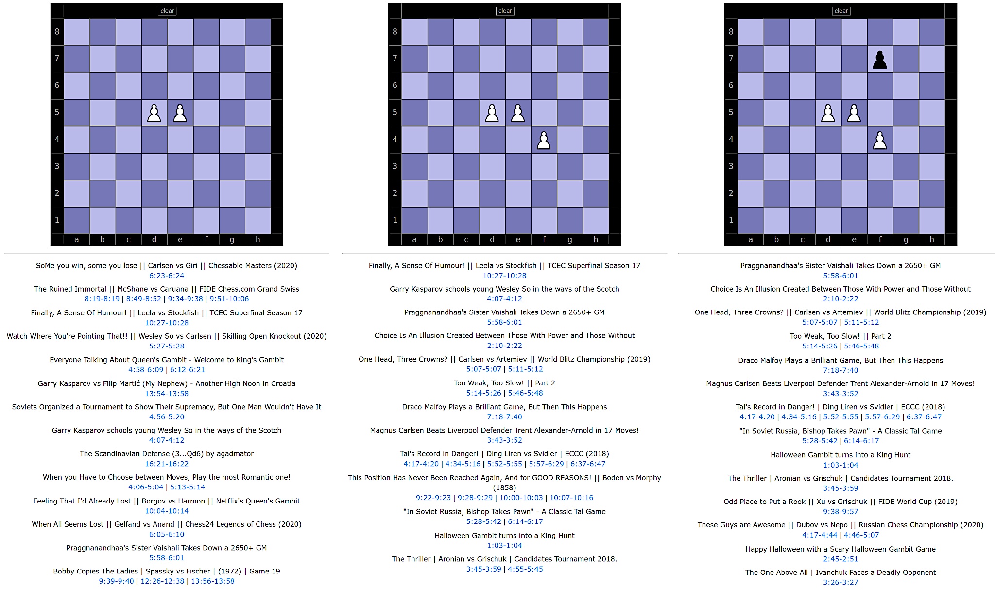
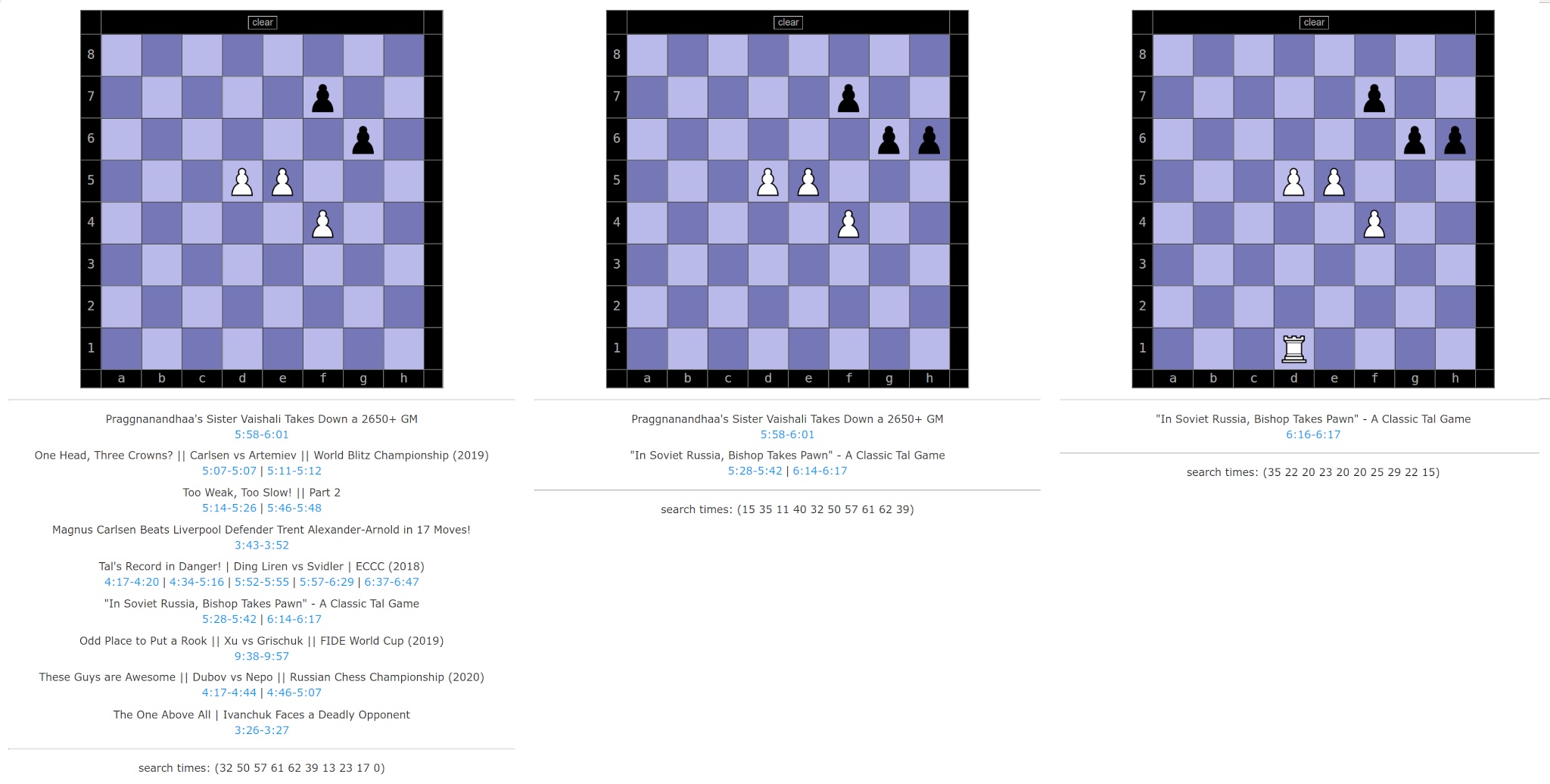
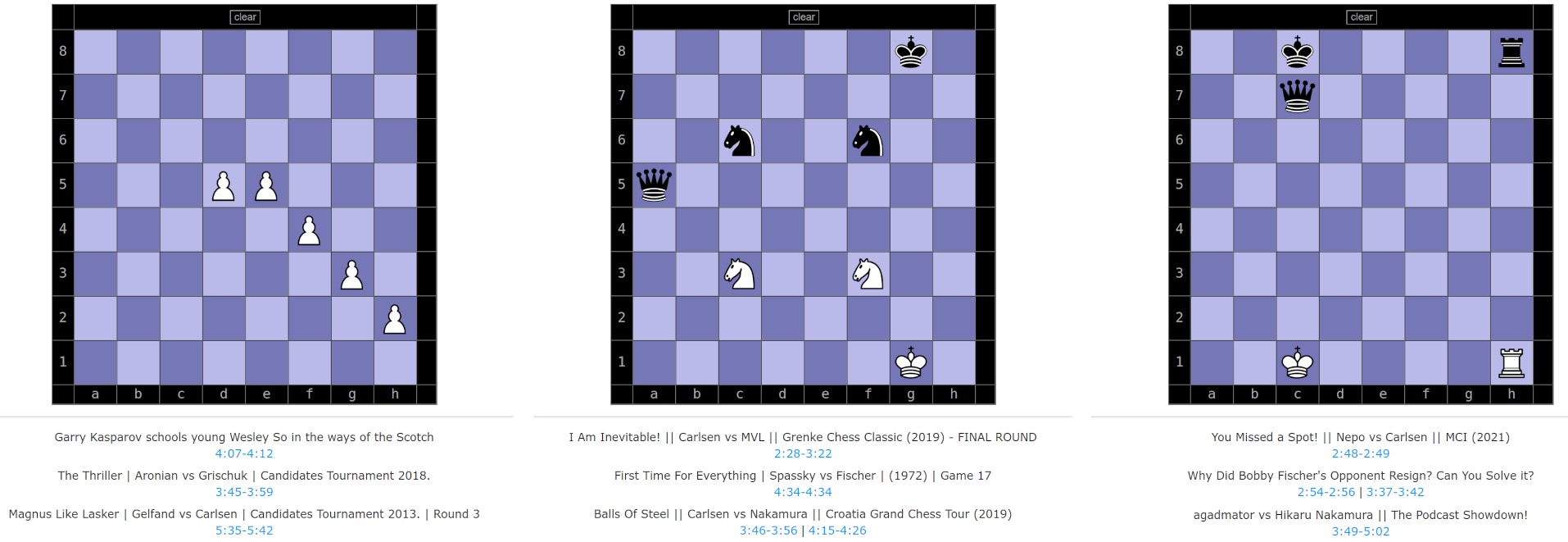
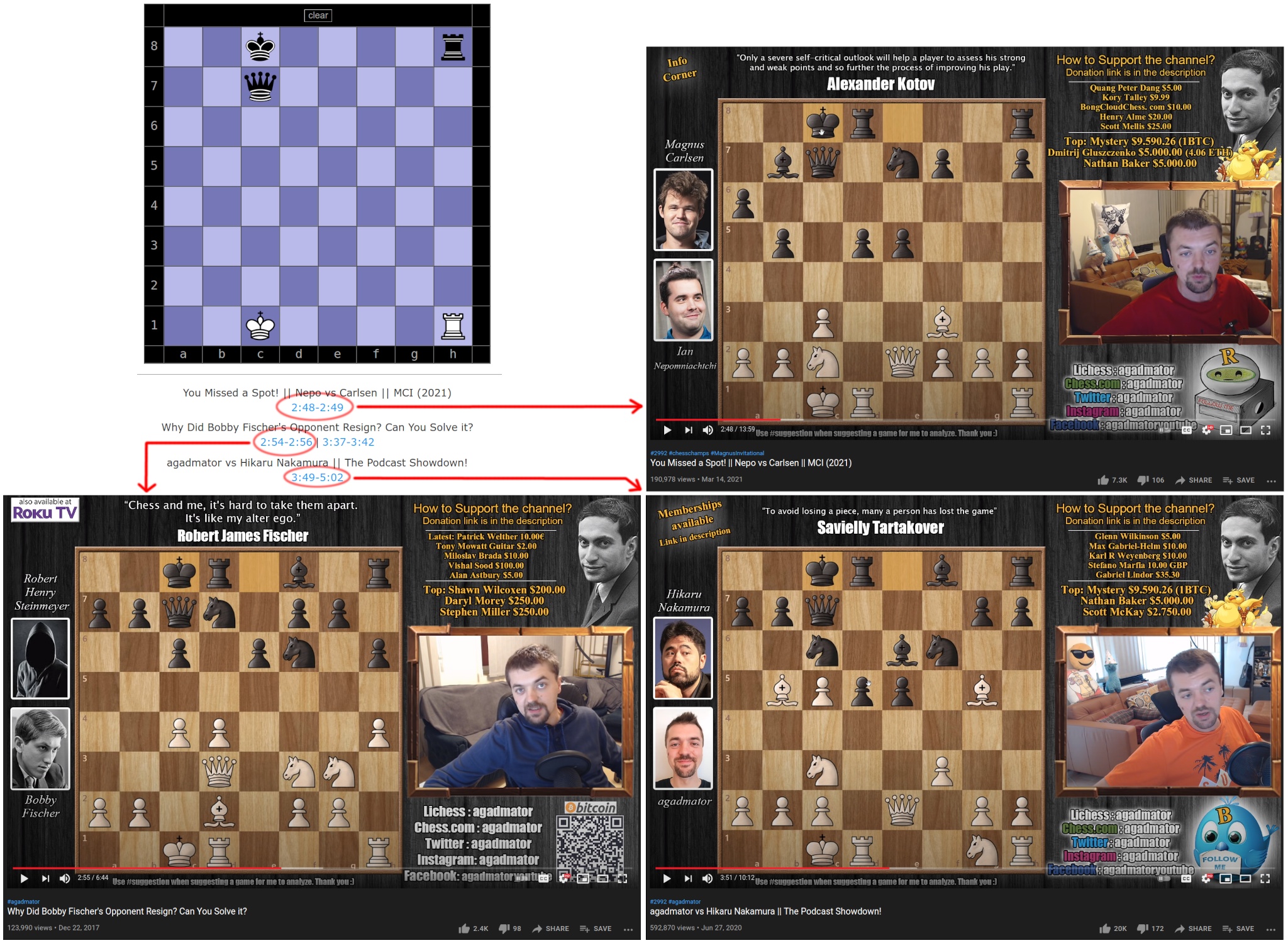
The UI is shown in fig­ures 13 - 16, along with links to videos of games match­ing (par­tially) to each board po­si­tion. At the mo­ment it has a ba­sic click-and-pick UI, lack­ing the per­haps ex­pected drag-and-drop sup­port. Nev­er­the­less it has the most im­por­tant ca­pa­bil­ity: find­ing match­ing games! Nat­urally as we place more and more pieces on the board a nar­rower set of videos match the query, this is shown in Fig­ures 13 and 14. The fi­nal po­si­tion matches just a few sec­onds of a sin­gle game, out of the 500 hours of con­tent.

The pro­ject is now more or lesss ready, but of course more im­prove­ments could be done. Firstly au­to­matic san­ity checks could be run on de­ter­mined board po­si­tions. For ex­am­ple we know that there must al­ways be one white and one black king on the board. Also typ­ically there are only one bish­ops on each square color (al­though a rare sub-pro­mo­tion is pos­si­ble). And pawns can­not ex­ist at the first or last rank, any such pieces are most likely mis-iden­ti­fied bish­ops.

A sec­ond set of im­prove­ments are re­gard­ing the UI. It doesn't have a drag-n-drop sup­port, free text search, video date fil­ter etc. But the ba­sic func­tion­al­ity is there, and it is very re­spon­sive since the search takes typ­ically just 5 - 50 mil­lisec­onds.

The third miss­ing fea­ture is au­to­matic up­dates, and this re­ally lessens the util­ity of this tool as time passes. Agad­ma­tor is con­stantly pro­duc­ing new con­tent, and even within a few months you can­not be sure whether you are see­ing just "par­tial" search re­sults. In­te­grat­ing the Keras model with AWS Lambda would be a very good ex­cer­cis, and I might do it at some point in fu­ture. Well, at least the UI should show when was the list time the database was up­dated. I am amazed if you have read all of this, even I can barely do it :D So as a re­minder, the code is hosted as at AWS S3.

---

Related blog posts:

Image and video clustering with an autoencoder, 2022 Jan (Matching: Autoencoder, Computer Vision, Keras, Python)
Introduction to Stable Diffusion's parameters, 2022 Nov (Matching: Autoencoder, Computer Vision, Python)
Cheating at Bananagrams with real-time AI, part 1, 2023 Apr (Matching: Computer Vision, Keras, Python)
Matching puzzle pieces together, 2022 Jul (Matching: Computer Vision, Keras, Python)
Helsinki Deblur Challenge 2021, 2021 Dec (Matching: Computer Vision, Keras, Python)