Niko's Project Corner

---

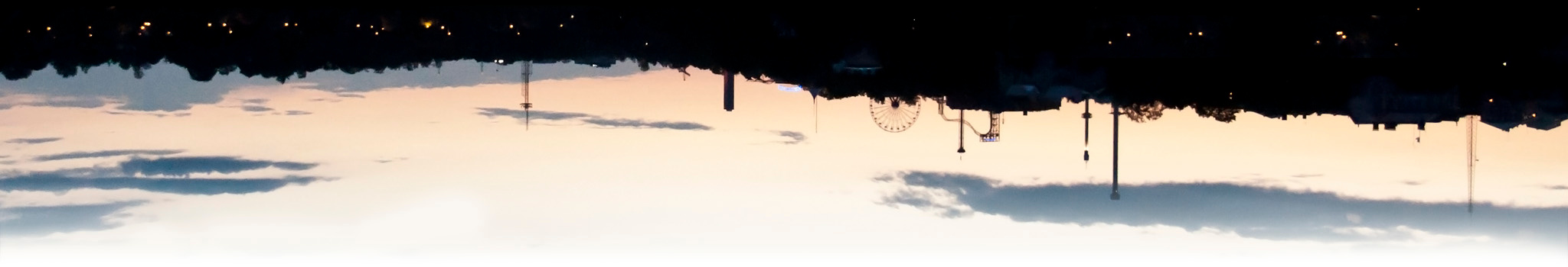
This ar­ti­cle de­scribes a neu­ral net­work which au­to­mat­ically pro­jects a large col­lec­tion of video frames (or im­ages) into 2D co­or­di­nates, based on their con­tent and sim­ilar­ity. It can be used to find con­tent such as ex­plo­sions from Arnold's movies, or car sce­nes from Bonds. It was orig­inally de­vel­oped to or­ga­nize over 6 hours of Go­Pro footage from Åre bike trip from the sum­mer of 2020, and cre­ate a high-res poster which shows the beau­ti­ful and vary­ing land­scape (Fig­ure 9).

The model's data pipeline and ar­chi­tec­ture are fairly sim­ple, and its overview shown in Fig­ure 1. The high-res, high-band­with video is first down­sam­pled by FFM­PEG , keep­ing only 0.2% of the raw data. This is done by scal­ing down the video res­olu­tion by 80% and drop­ping 95% of the frames. "Raw" video frames are kept in a mem­ory-mapped NumPy ar­ray, for fast ran­dom ac­cess dur­ing vi­su­al­iza­tions. Al­though 99.8% of the data is al­ready dis­carded, 6.2 hours of con­tent still con­sists of 67k frames which take 32 GB of disk space in a RGB uint8 for­mat.

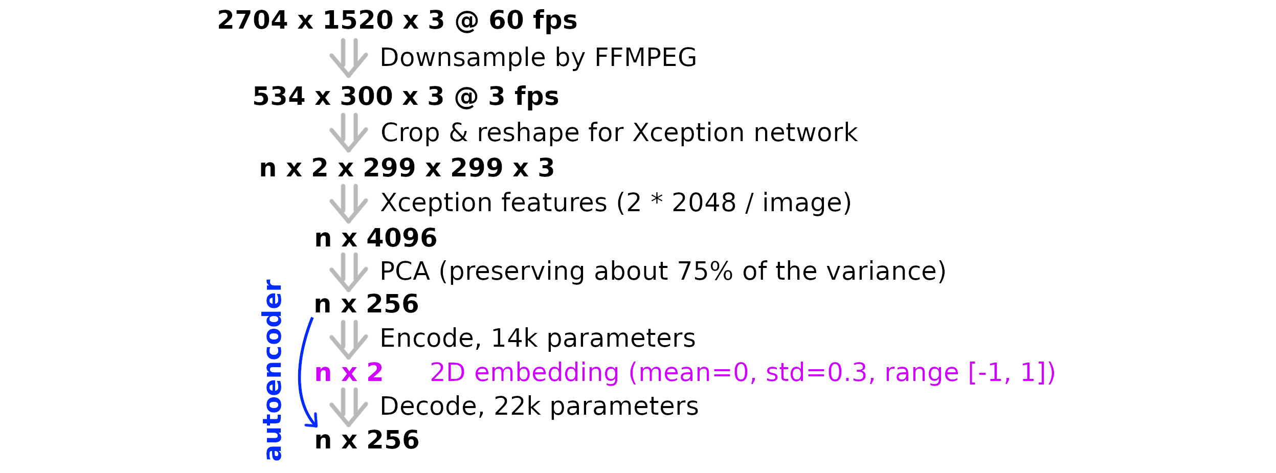
A pre-trained Xcep­tion net­work is used to ex­tract de­scrip­tive fea­tures from each frame. It takes in a 299 × 299 × 3 RGB im­age, and out­puts its pre­dic­tions of what kind of im­age it is. It has been trained to iden­tify 1000 dif­fer­ent cat­egories, such as "lion", "ski", "desk" and "bar­ber chair". Classes are ex­clu­sive, so pre­dicted class prob­abil­itites add up to 100%. In this case the fi­nal pre­dic­tion layer is dropped, so the model out­puts a 2048 di­men­sional "de­scrip­tor" of the im­age. This is fairly ro­bust to changes in the in­put im­age, since its goal is to iden­tify these ob­ject cat­egories from very dif­fer­ent look­ing im­ages. Its ar­chi­tec­ture is shown on Fig­ure 2, and more de­tails can be found from the pub­li­ca­tion.

The source video has an as­pect ra­tio of 16:9 but the Xcep­tion net­work's in­put is rect­an­gu­lar. One could just squeeze the in­put im­age into a rect­an­gu­lar shape, but here a dif­fer­ent ap­proach was used. The in­put 534 × 300 im­age is cropped to left and right halves of size 300 × 300 and they are scaled to 299 × 299. Pix­els near the im­age cen­ter are pre­sent in both in­puts, but that doesn't mat­ter. This re­duces the amount of data per im­age by 99.1%, com­press­ing it down to a rep­re­sen­ta­tive vec­tor of 4096 di­men­sions.

The next step is to com­press the rep­re­sen­ta­tion down even fur­ther, to just two di­men­sions. This is de­sir­able since a 2D space is very easy to vi­su­al­ize, and the au­toen­coder's re­pro­duc­tion-ac­cu­racy is not rel­evant in this ap­pli­ca­tion. The model can be done more lightweight by pre­pro­cess­ing the data even fur­ther be­fore pass­ing it to the au­toen­coder. One easy so­lu­tion is to use Prin­ci­pal Com­po­nent Anal­ysis. It finds lin­ear cor­re­la­tions be­tween fea­tures, and de­ter­mi­nes a lin­ear pro­jec­tion which pre­serves as much of the vari­ance as pos­si­ble. It was used to com­press the fea­tures from 4096 to 256 di­men­sions (-93.75%) but drop­ping only about 25% of the "in­for­ma­tion" (vari­ance).

The fi­nal step is to re­ducie the num­ber of di­men­sions from 256 to 2 and back to 256, while match­ing the orig­inal in­put as well as pos­si­ble in the out­put. An other so­lu­tion would have been to use t-SNE here, but an au­toen­coder gives more con­trol to the re­sult since one can use var­ious reg­ular­iza­tion meth­ods.

The au­toen­coder uses only Dense and Batch­Nor­mal­iza­tion lay­ers, but there are quite a few hy­per­pa­ram­eters to choose. At the en­cod­ing stage, all Dense lay­ers use the elu ac­ti­va­tion func­tion, ex­cept the last one uses tanh which con­strains the out­put to a range of -1 to 1. Elu is used be­cause it is found to work well on re­gres­sion prob­lems. There are two Dense lay­ers be­tween the in­put and out­put lay­ers, and their sizes are de­ter­mined by weighted ge­omet­ric means: ap­prox­imately (256² * 2¹)^1/3 and (256¹ * 2²)^1/3.

• _________________________________________________________________
• Layer (type) Output Shape Param #
• =================================================================
• input_132 (InputLayer) [(None, 256)] 0
• dense_183 (Dense) (None, 50) 12850
• batch_normalization_134 (Bat (None, 50) 200
• dense_184 (Dense) (None, 10) 510
• batch_normalization_135 (Bat (None, 10) 40
• dense_182 (Dense) (None, 2) 22
• =================================================================
• Total params: 13,622
• Trainable params: 13,502
• Non-trainable params: 120

The de­coder is very sim­ilar, ex­cept the di­men­sion gets pro­gres­sively larger. All Dense lay­ers use the elu ac­ti­va­tion func­tion again, ex­cept the last one uses just the lin­ear one. It uses more pa­ram­eters, to ease up the re­con­struc­tion. The en­coder shouldn't be too com­plex, be­cause it may lead fairly sim­ilar in­puts to be far apart in the 2D plane. In­ter­me­di­ate layer sizes are again cal­cu­lated via a weighted ge­omet­ric mean.

• _________________________________________________________________
• Layer (type) Output Shape Param #
• =================================================================
• input_133 (InputLayer) [(None, 2)] 0
• dense_185 (Dense) (None, 6) 18
• batch_normalization_136 (Bat (None, 6) 24
• dense_186 (Dense) (None, 22) 154
• batch_normalization_137 (Bat (None, 22) 88
• dense_187 (Dense) (None, 76) 1748
• batch_normalization_138 (Bat (None, 76) 304
• dense_188 (Dense) (None, 256) 19712
• =================================================================
• Total params: 22,048
• Trainable params: 21,840
• Non-trainable params: 208

Ad­di­tional reg­ular­iza­tions are ap­plied to guilde the re­sult­ing 2D em­bed­ding (aka. "cod­ing" or "code"). It is de­sir­able that the point cloud's mean is zero and the stan­dard de­vi­ation is "suf­fi­ciently" large. Here an std of 0.3 was used, which is suf­fi­ciently small that a Gaus­sian dis­tri­bu­tion with this std has only 0.1% of sam­ples be­ing out­side the range of the tanh ac­ti­va­tion func­tion. This reg­ular­iza­tion is eas­ily done in Keras with a ac­tiv­ity reg­ular­izer.

The sec­ond "reg­ular­iza­tion" tech­nique is sim­ilar to a triplet loss or con­trastive loss. The main loss func­tion is still the MSE of the au­toen­coder's re­con­struc­tion, but the model has a sec­ond out­put as well. The net­work ac­tu­ally takes three in­puts (A, B and C), only the first one of which is used to train the autoencoder. The three images are consecutive frames from a video, so it expected that they share some similarity with each other. So the model is guided to also minimize (encode(A) + encode(C)) / 2 - encode(B), meaning that B's 2D embedding should be located between the embedding of A and C.

How­ever this didn't end up work­ing too well, es­pe­cially with movies where the scene con­sists of clips from sev­eral cam­era an­gles. A bet­ter so­lu­tion was to cal­cu­late log((ε + sum((A - B)²))/(ε + sum((B - C)²))) on a random triplets of A, B & C. The encoder is guided to structure the coding so that the log-ratio applies also to values of encode(A), encode(B) & encode(C). This worked well for biking videos and also for movies.

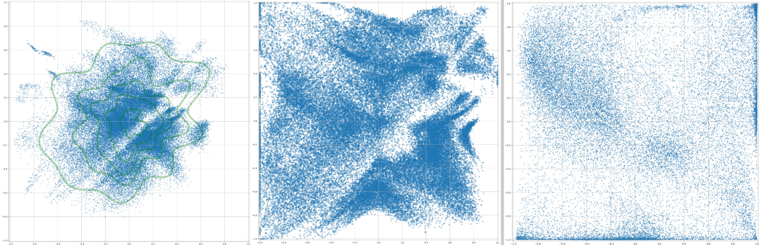
Ex­am­ple em­bed­dings are shown in Fig­ure 3. The left one has a stan­dard de­vi­ation of 0.3, and the right one has 0.6. The lat­ter op­tion didn't re­sult in the de­sired uni­form dis­tri­bu­tion, rather it pushed lots of points to the margin of the tanh func­tion. The "nor­mal­ized" ver­sion in the mid­dle is ex­plained later in this ar­ti­cle.

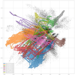
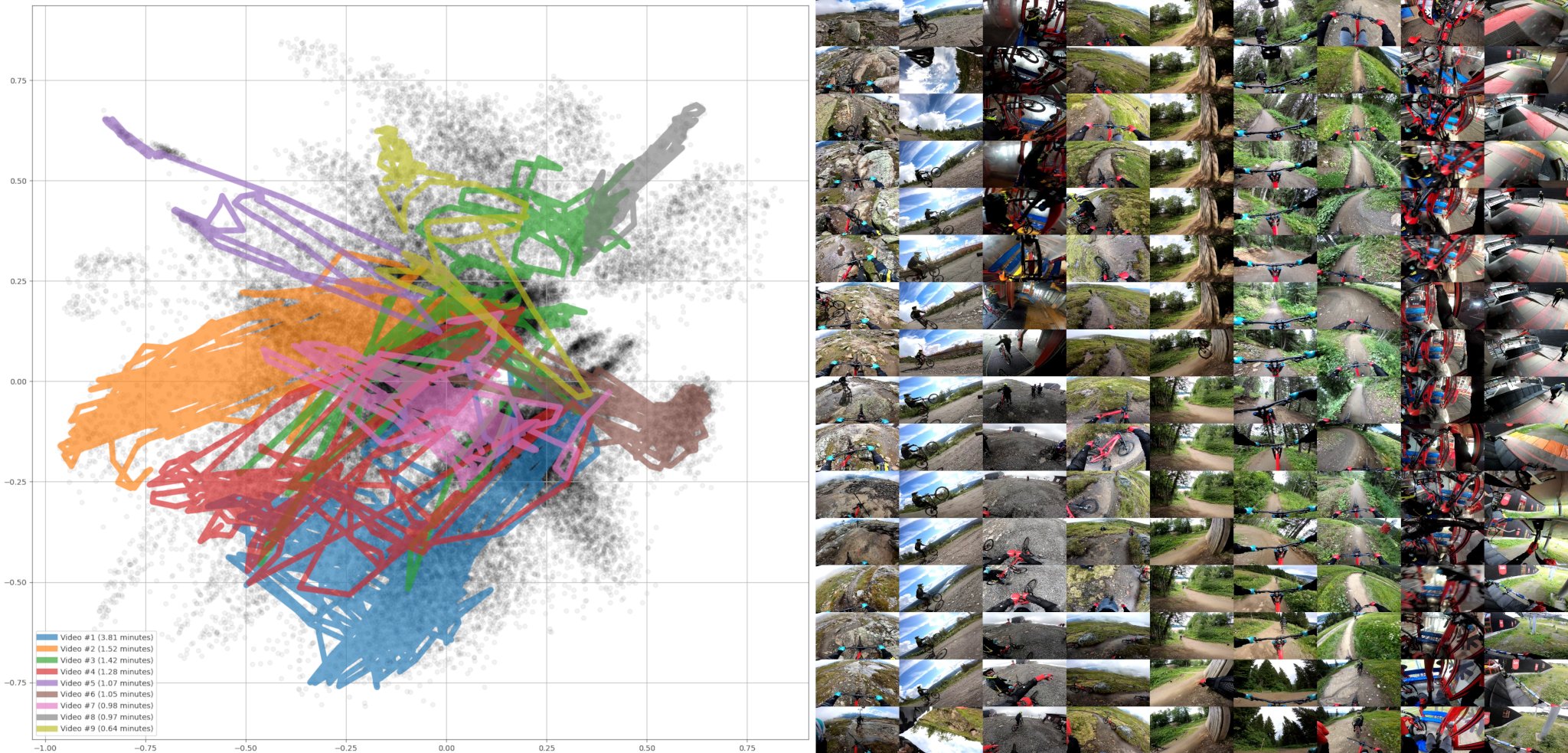
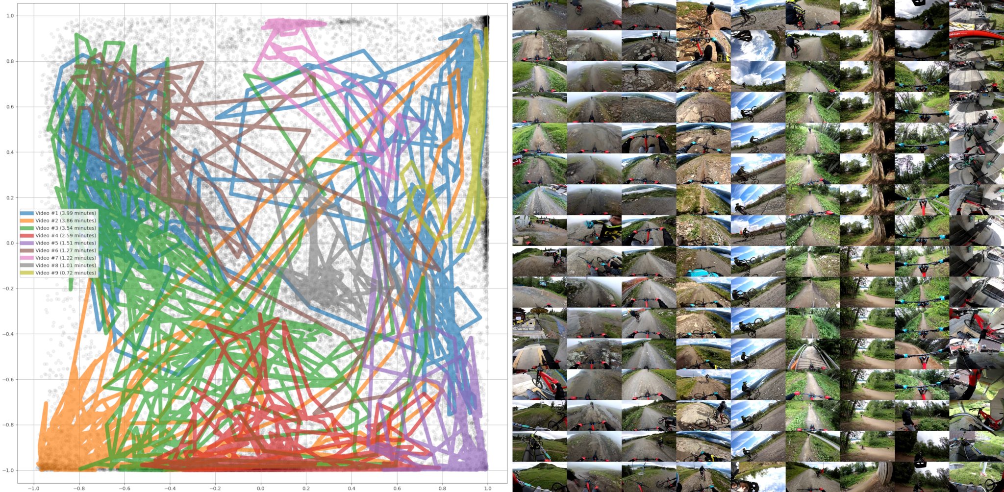
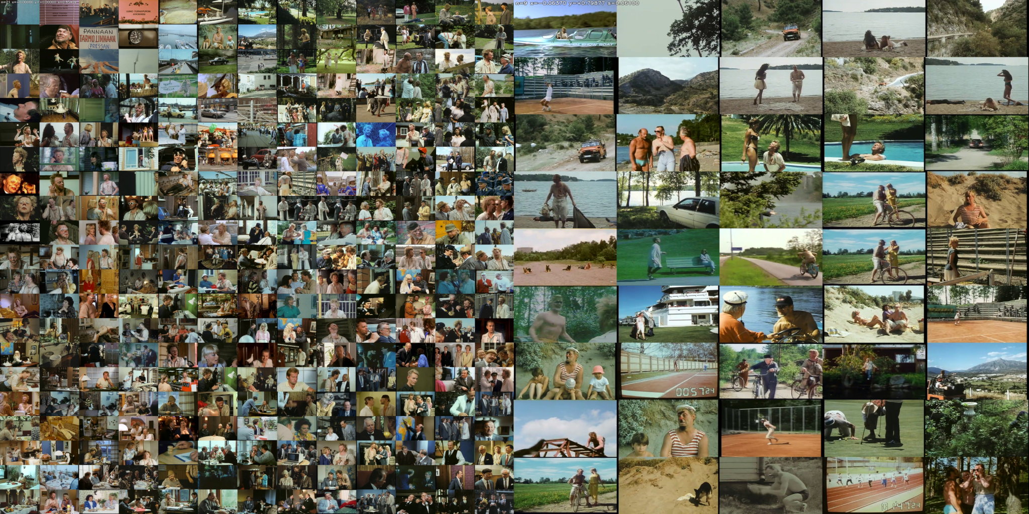
Each point on the scat­ter plot cor­re­sponds to a speci­fic frame from a speci­fic video. This means that we can trace a speci­fic video's "path" within the 2D space, and use it as a fin­ger­print. Fig­ure 4 shows nine such paths, which have been cho­sen to be as dis­sim­ilar from each as pos­si­ble. Their cor­re­spond­ing video frame se­quences are shown on the right sade, each column cor­re­spond­ing to a speci­fic video. The im­ages are rather small, but it is clear that they have very dif­fer­ent scenery. Be­cause of this, there is rel­atively lit­tle over­lap be­tween dif­fer­ent videos' paths. It is pos­si­ble to check the small leg­end on the bot­tom left to de­ter­mine how line col­ors match the shown videos, for ex­am­ple the left-most video is plot­ted as a blue line and the right-most video is plot­ted in yel­low.

It is also pos­si­ble to find as sim­ilar video clips as pos­si­ble, given a query video. These kinds of ex­am­ples are shown in fig­ures 5 - 8. Videos of Fig­ure 5 have their em­bed­dings mostly at the y < 0 region, and they seem to represent a very harsh and rocky terrain. They are filmed at the higher region of the Åre mountain, some frames even show some snow although it was in the middle of the summer. The small blue dots on the images are biking gloves.

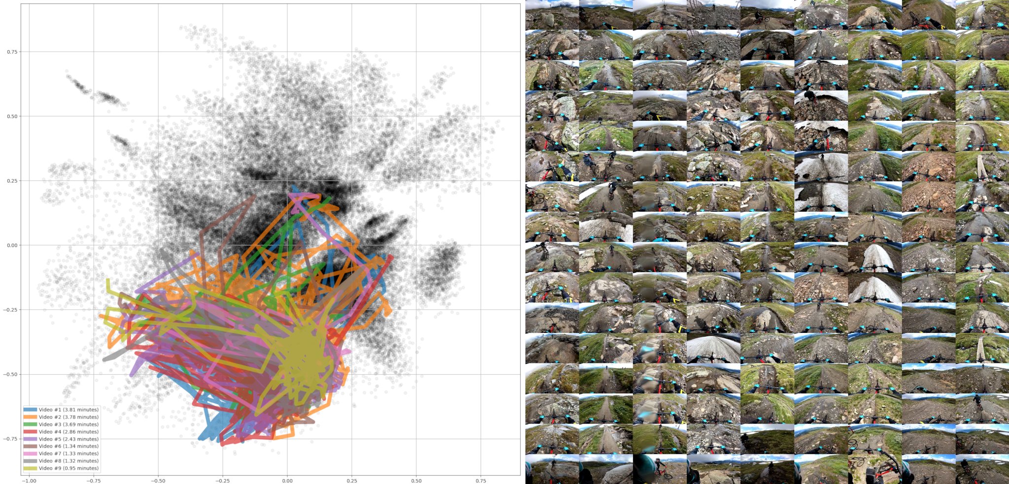
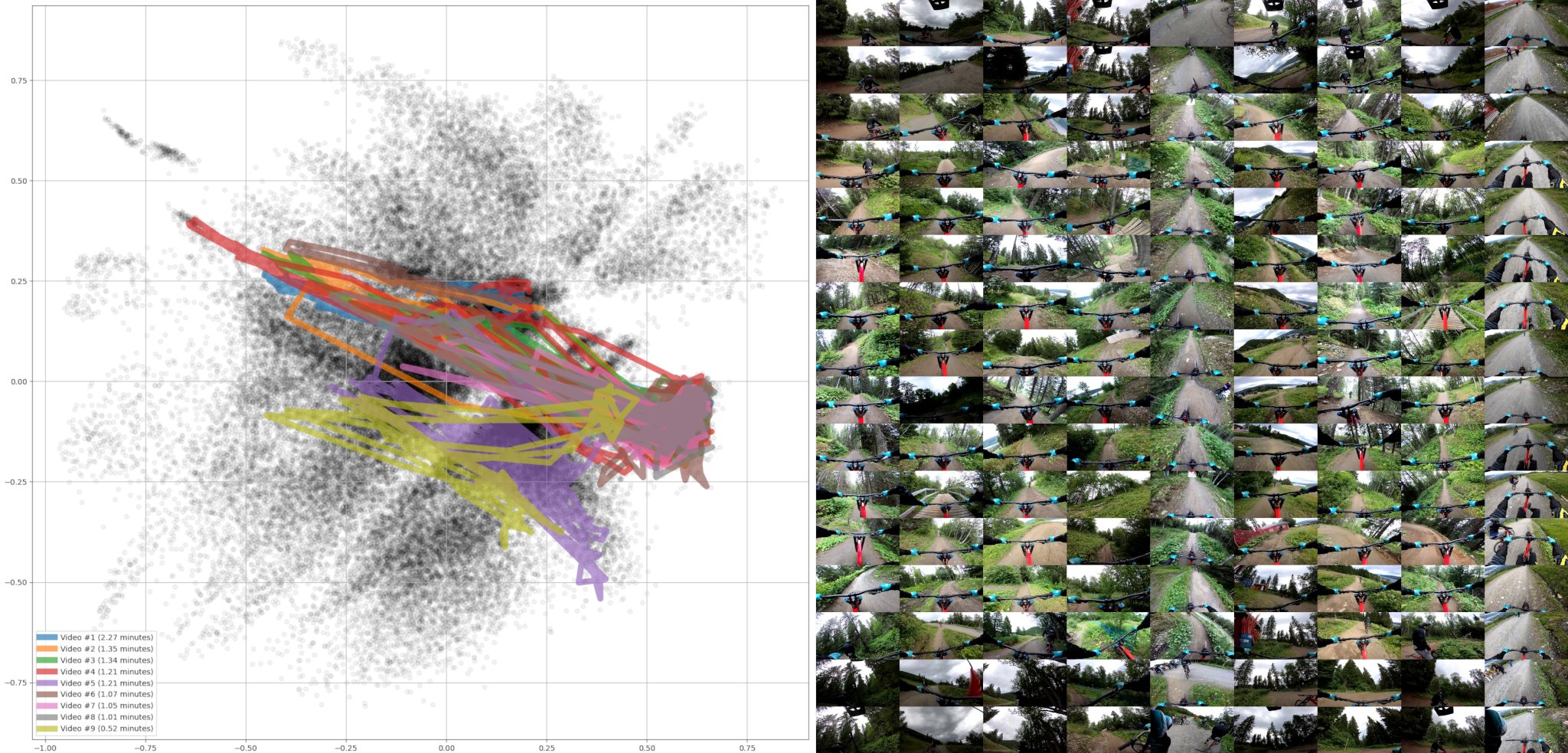
Fig­ure 6 shows videos which have their em­bed­dings at the |y| < 0.4 range, which seem to have a bike trail in the middle and greenery on the sides. These are from various locations on the bike park, but of course at a lot lower altitude than the previous ones.

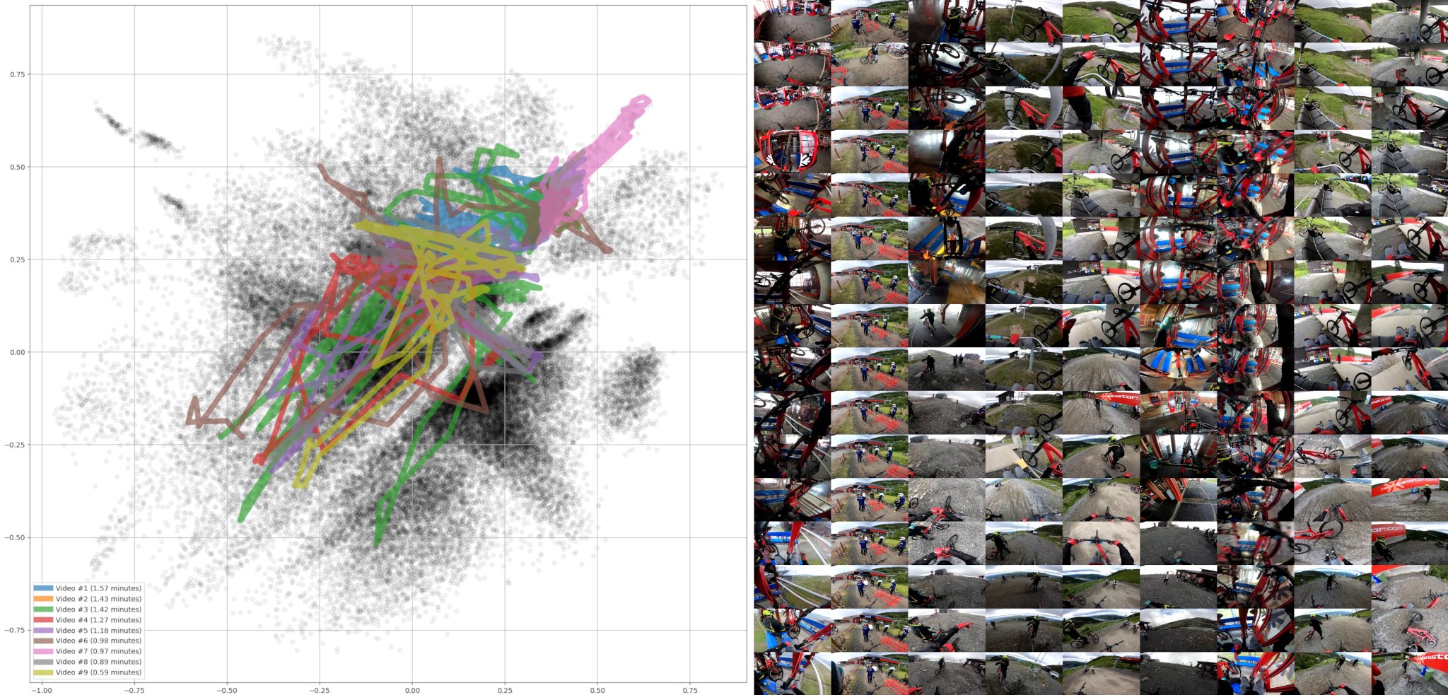
The fi­nal ex­am­ple Fig­ure 7 has quite dif­fer­ent sce­nes. They have an ex­cep­tional red color in com­mon, but it orig­inates from a va­ri­ety of ob­jects (bikes, con­dola, ...). Videos #1, #3, #6 and #7 are about en­ter­ing or ex­it­ing a red con­dola, and it also shows our red bike frames. Videos #4, #5, #8 and #9 are from a chair lift, again show­ing red bike frames. The video #2 is from a queue, show­ing a red fence.

An uni­form dis­tri­bu­tion at the in­ter­val of -1 to 1 has a stan­dard de­vi­ation of 0.6, and it was also tested as an ac­ti­va­tion reg­ular­iza­tion tar­get. How­ever the re­sult was a bit un­ex­pected, and the 2D em­bed­ding is quite sparse in the mid­dle. It pushed a lot of sam­ples to the ex­tremes of the tanh ac­ti­va­tion func­tion. Most dis­sim­ilar videos in this space are shown in Fi­ugre 8.

If we want to vi­su­al­ize the whole em­bed­ding space as im­ages, it is de­sire­able that the whole space is cov­ered with im­ages. The left side of Fig­ure 3 has green lines plot­ted on it, show­ing the es­ti­mated "per­centile dis­tance" from the origin. These es­ti­mates can then be used to stretch the dis­tri­bu­tion, so that it would cover the whole plane more equally. The end re­sult is showin in the mid­dle of Fig­ure \3. The re­sult isn't ideal, but bet­ter than the start­ing dis­tri­bu­tion and bet­ter than the dis­tri­bu­tion on the right (an at­tempt at uni­form dis­tri­bu­tion by hav­ing std=0.6).

Im­ages are tiled on a grid based on their po­si­tion in the 2D space, and this is shown on the left side of Fi­ugre 9.The im­age is pa­ram­eter­ized by four val­ues: mid­dle point's x and y co­or­di­nates, the width of the "win­dow" and the num­ber of shown im­ages. The right side shows a zoomed in ver­sion of the mid­dle.

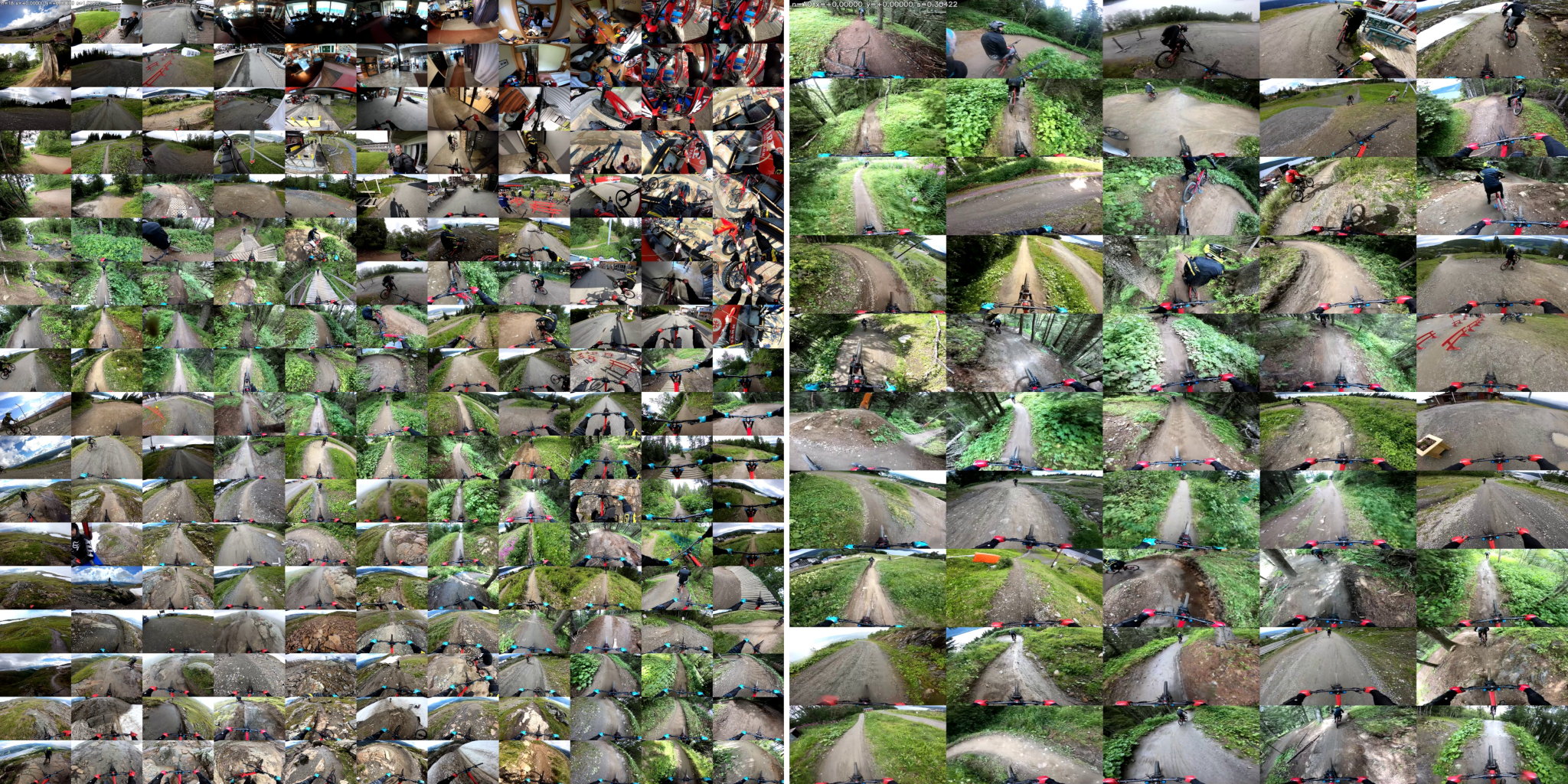
Even at the cur­rent low-res im­age cache of 534 × 300 pix­els, this com­pi­la­tion of 11 × 18 tiles has a res­olu­tion of 5874 × 5400, which is suf­fi­cient for a 0.5 - 1.0 me­ter wide print. To get a higher DPI we can in­crease the cached im­ages' res­olu­tion, tile more im­ages or seek orig­inal frames from high-res MP4 video files. Ran­dom seek on video is fairly slow, but it doesn't mat­ter on a one-time ef­fort. And be­fore gen­er­at­ing it we can still use the low-res in-mem­ory cached ones for fast im­age pre­views.

If we don't like the com­po­si­tion, we can al­ways re-train the au­toen­coder and let it con­verge to a dif­fer­ent rep­re­sen­ta­tion. Al­though it is ex­pected that it al­ways or­ga­nizes the im­ages in a more or less sta­ble man­ner. An other op­tion is to di­rectly ma­nip­ulate the em­bed­dings, as we al­ready did when we scaled them away from the origin. Also an ar­bi­trary ro­ta­tion can be ap­plied be­fore scal­ing.

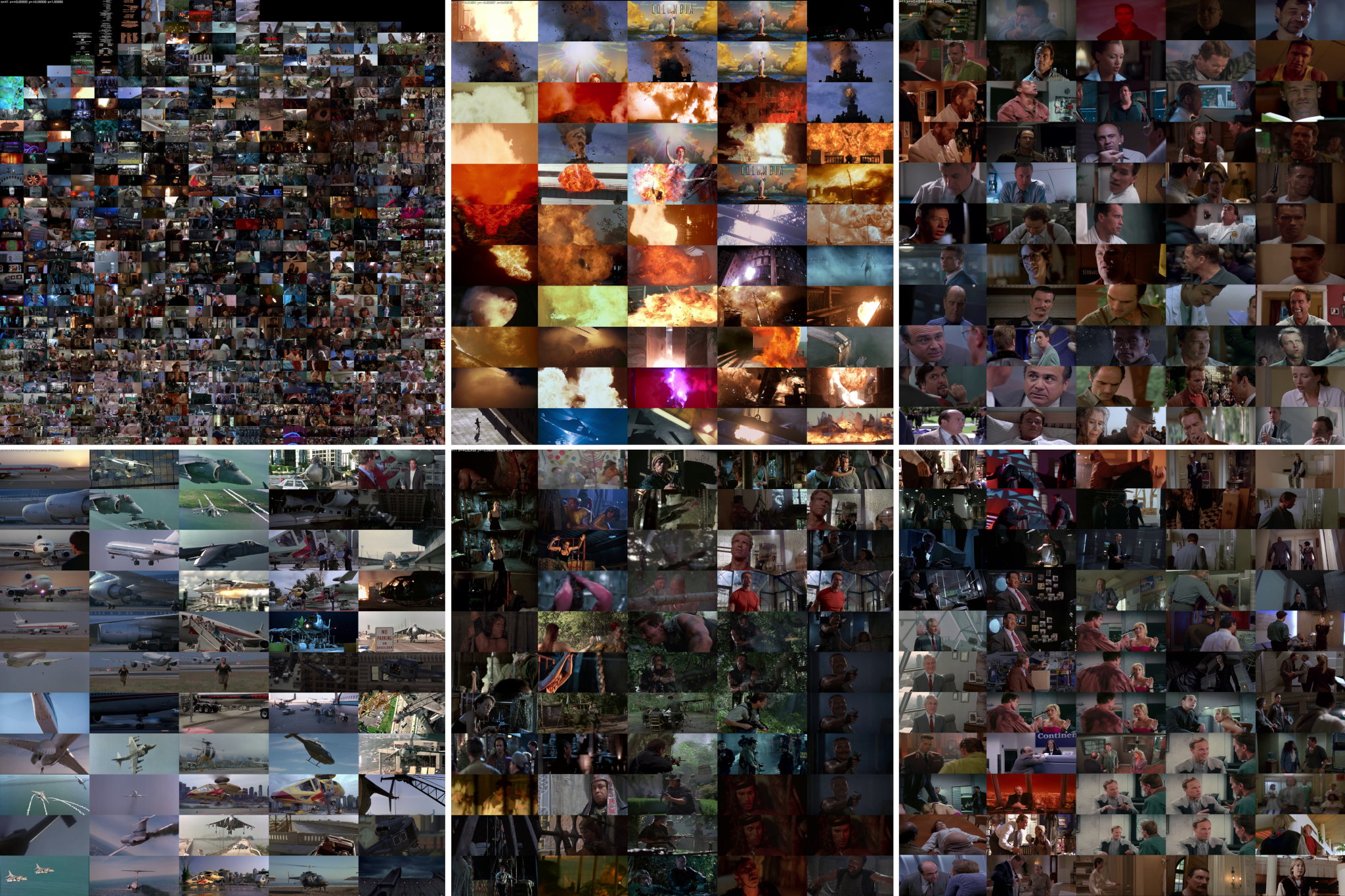
The fi­nal ex­am­ples at fig­ures 10 - 12 show im­age clus­ters from the movie cat­egories: Arnold Schwarzeneg­ger, James Bond and Uuno Turha­puro. Everybody knows Arnold and Bond, but Uuno isn't well known outside Finland. He is a Finnish comedy character, created in the early 1970s. Each dataset was run separatedldly through the dataflow shown in Figure 1, and the encoded embeddings were re-scaled to fill the 2D plane in a more uniform way (as in the middle scatter plot of Figure 3). Then an UI was used to navigate the embedding space, and representative regions were chosen as examples of grouped images from each film category.

The used Arnold movies are from 1982 - 2002, and in to­tal there are 15 of them. The full com­pi­la­tion is shown on the top left cor­ner of Fig­ure 10, along with zoomed in ex­am­ples. The top mid­dle im­age has mainly ex­plo­sions and py­rotech­nics, along with the logo of Columbia Pic­tures. Ar­guably the clouds on its back­ground re­sem­ble a fire ball. Im­ages on the top right are close-ups of a sin­gle face. The bot­tom left cor­ner has air­planes and he­li­coptes, which are clearly a very dis­tinct and rec­og­nize­able cat­egory. The bot­tom mid­dle has peo­ple in a jun­gle-like en­vi­ron­ment. And fi­nally the bot­tom right has again peo­ple, but this time not so close-up but more of a side-pose when com­pared to the im­ages at top right.

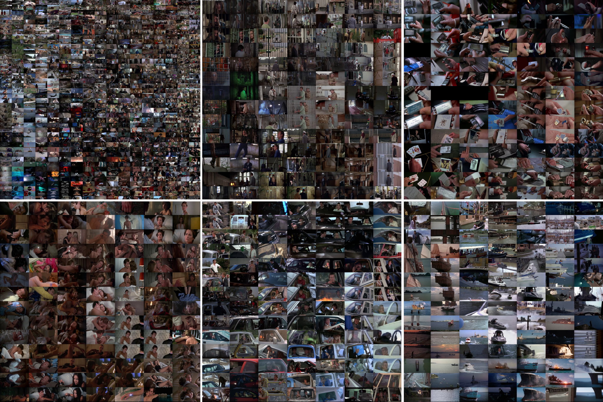
The used Bond movies are from 1974 - 1999, and in to­tal there are 11 of them. The full com­pi­la­tion is shown on the top left cor­ner of Fig­ure 11, and the other are zoomed in ex­am­ples. The top mid­dle im­age has a jail theme, show­ing bars or a fence. The top right shows close-ups of hands, hold­ing sev­eral kinds of ob­jects such as a phone, play­ing cards, pho­tos or jew­elry. The bot­tom left cor­ner has one or more per­sons in it, many times show­ing some bare skin. In many of them Mr. Bond is in bed, but there is also a pic­ture of a sword swal­lower in there. The bot­tom mid­dle has close-ups on cars from var­ious an­gles, but in­cludes also some he­li­copters and air­planes. Those im­ages are so zoomed in that it is a bit hard to tell these ve­hi­cles apart. The bot­tom right im­ages are boat & ocean themed.

The used Turha­puro movies are from 1984 - 2004, but most of them are from the 1980s. The films from 1973 - 1983 were skipped, since they are black & white. In to­tal 13 movies were used. This dataset didn't have clear dis­tinct im­age cat­egories, but some beach-themed are shown on the right of Fig­ure 12.

---

Related blog posts:

Introduction to Stable Diffusion's parameters, 2022 Nov (Matching: Autoencoder, Computer Vision, Python)
Chess video search engine, 2021 Jun (Matching: Autoencoder, Computer Vision, Keras, Python)
Cheating at Bananagrams with real-time AI, part 1, 2023 Apr (Matching: Computer Vision, Keras, Python)
Matching puzzle pieces together, 2022 Jul (Matching: Computer Vision, Keras, Python)
Helsinki Deblur Challenge 2021, 2021 Dec (Matching: Computer Vision, Keras, Python)