
The Finnish Inverse Problems Society (FIPS) organized the Helsinki Deblur Challenge 2021 during the summer and fall of 2021. The challenge is to "deblur" (deconvolve) images of a known amount of blur, and run the resulting image through and OCR algorithm. Deblur-results are scored based on how well the pytesseract OCR algorithm is able to read the text. They also kindly provided unblurred versions of the pictures, so we can train neural networks using any supervised learning methods at hand. The network described in this article isn't officially registered to the contest, but since the evaluation dataset is also public we can run the statistics ourselves. Hyperparameter tuning got a lot more difficult once it started taking 12 - 24 hours to train the model. I might re-visit this project later, but here its status described as of December 2021. Had the current best network been submitted to the challenge, it would have ranked 7th out of the 10 (nine plus this one) participants. There is already a long list of known possible improvements at the end of this article, so stay tuned for future articles.
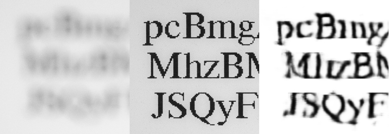
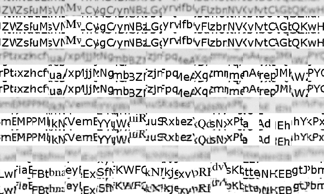
In total 17 teams registered to the contest, all of which seem to be from an university. I expected more individual participants, which is the case in most Kaggle competitions. The dataset is of a very high quality, and clearly lots of thought went into its design. It consists of 20 different levels of blur, each of which has 200 pictures. Each photograph shows unique strings, photographed by two cameras. One camera is always kept in focus, while the other is progressively adjusted to be out of focus. More detail can be found from their paper. A cropped example for the input, the target and a network's output is shown in Figure 1.
In total there are 20 × 200 × 2 = 8000 images, each of which is 2360 × 1460 = 3.45 megapixels. In the TIFF format they take 57 GB of space (grayscale, 16 bits of precision), which seem to use lossless compression. To actually feed them to the neural network they need to be converted into a "raw" numpy array, typically in-memory. We can save a significant amount of space by keeping just 8-bits of precision, then each image takes 3.45 MB of RAM. Multiplying this by 8000 images it still pushes the RAM requirement to 28 GB, which might not be feasible on a typical desktop. Luckily there are many ways around this.
At first we can reduce the image resolution, since the e-ink display's pixels seem to correspond to about 8 pixels in the photo. So each image can be scaled down by 1 : 4 - 1 : 8, reducing the memory requirement by 94 - 98\%! A high-res dataset is nice but we don't need that many pixels for the OCR algorithm to work. Actually even the official evaluation script scales images down by 50% to improve OCR results.
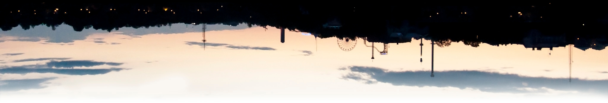
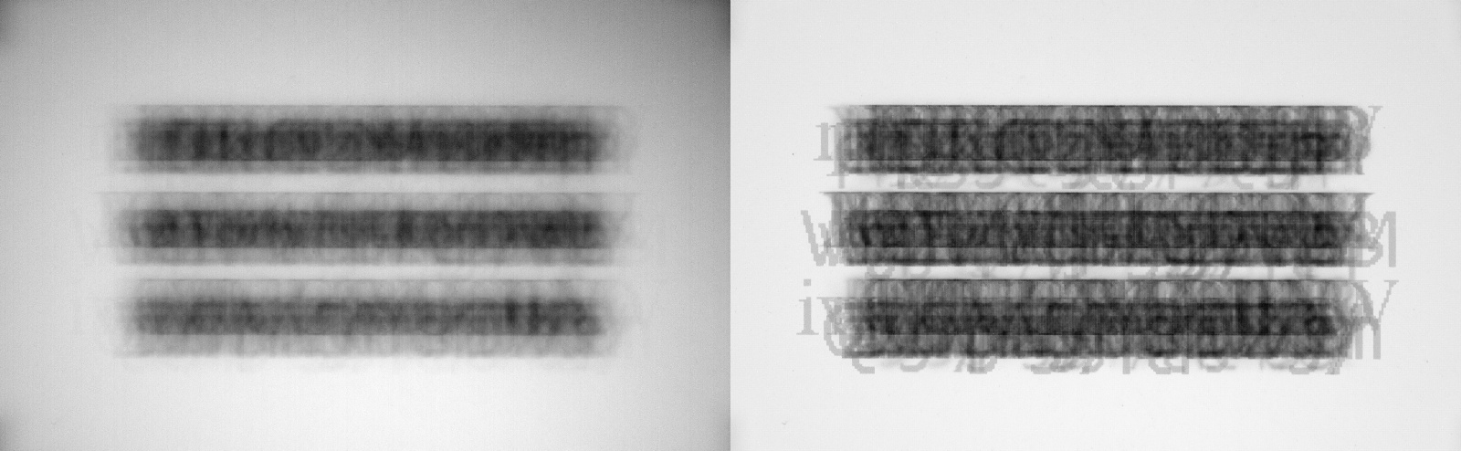
The other option is to crop the images further, leaving out the borders which don't contain any text. This was originally implemented, but it was later found out that the algorithm confused blurred dark corners (vignetting, see Figure 2) with heavily blurred text, and produced dark artefacts around the intended text area. This wouldn't be that much of an issue for a human, but the OCR mistook these for characters and generated more than the intended three lines of text as the output. This caused the score to plummet to zero, since no characters were correctly matched with the known correct output. This is apparent in some examples of models' outputs, as shown in Figure 3.
At this point the discovery process is not narrated in a chronological order, rather the article describes how the final version of the data processing pipeline and the neural network works.
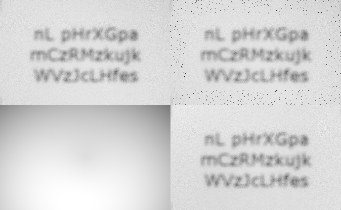
Each image is scaled down by a factor of 1 : 7, dropping the resolution from 2360 × 1460 to 337 × 208. This leaves characters' details at a width of just 0.5 - 4 pixels, which might actually be a bit too small. To midigate the issue with vingetting, each input image goes through a process of estimating the background brightness at each pixel and then having it subtracted. This is achieved by fitting a low-degree polynomial f(x, x2, y, y2, d), where x & y are the image coordinates and d is the distance from the image's center. Only pixel values near the border are used to fit this function, because they are known not to contain any text. A robust least-squares estimate is obtained by first fitting the model to all the data and then discarding the top 10% of data which does not fit the model. These steps are shown in Figure 4. Not all of the 30.000 border pixels (about 40% of the image area) are needed to fit the simple function, a sufficiently large sample of 400 - 450 pixels was used.
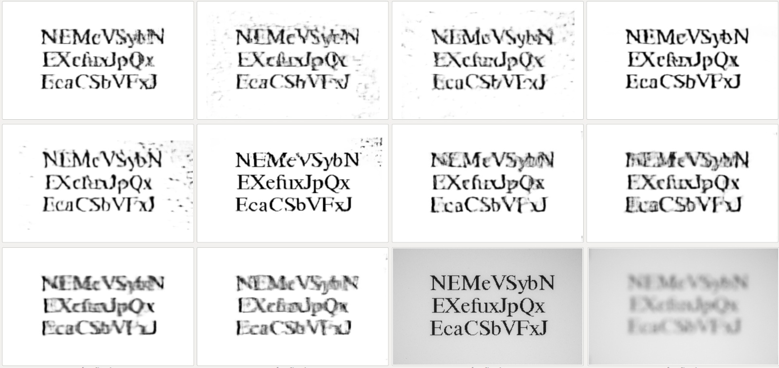
If the input is just a grayscale image, the first few convolution layers wouldn't have that many interesting features to extract. This network utilizes a non-linear median filter with a width of 3, 5, 7 and 9 pixels to augment the input image. Not much hyperparameter-tuning was done on this, but overall it improved results. Examples of these median-filtered images are shown in Figure 5. Maybe this many small steps is overkill, and widths of just 3 and 7 pixels is sufficient. Although now it seems obvious that these filters have the most effect on the least blurred images, and those are the easiest to deblur anyway.

There is also a significant amount of preprocessing done to the target "ground truth" (sharp) images. Their background is not completely white, but rather at 80 - 85% brightness. However the model's last activation is sigmoid, which scales the output to a number between zero and one. Also on previous projects (at least on a face VAE, not in this blog yet) it was discovered that binary_crossentropy produces sharper images than MSE. So the target images were re-scaled so that 75% of the pixels are at 100% brightness. Again mild vingetting started causing issues, but on this context it was midigated in a very different manner than with the blurred images.
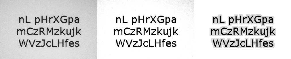
On the target image, non-white pixels (e.g. black or grayscale) are allowed only near completely black pixels. Vingetting isn't so extreme that the corners would have even a single black pixel, only gray. These are still suboptimal for the network's loss function and the OCR step so it is best to fix them. This simple heuristic works very well, as is shown on Figure 6.
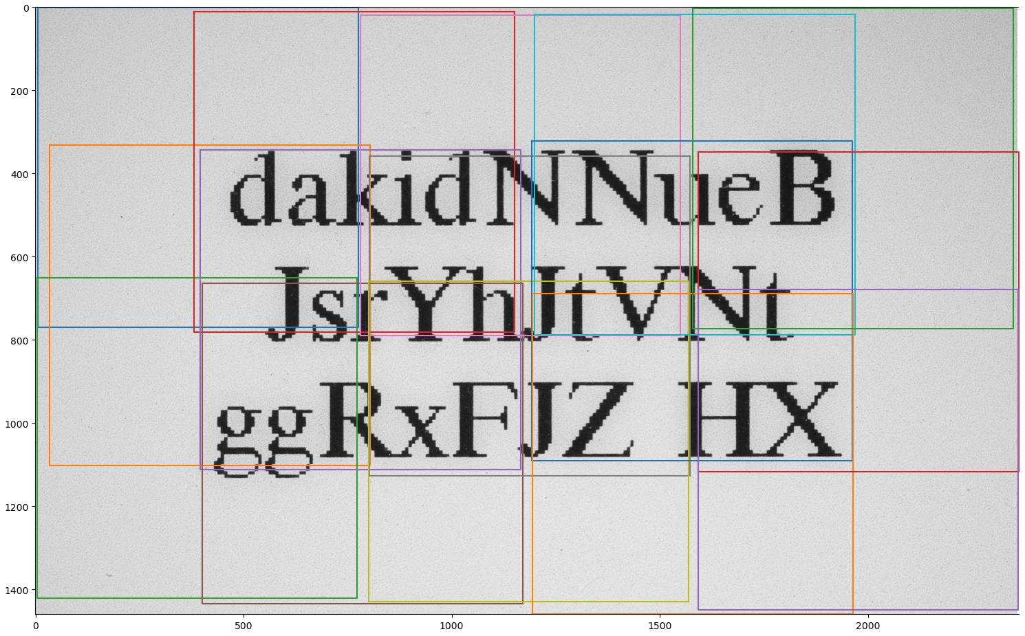
Training the network puts a very heavy load on the GPU, and caused UI programs to lag. This isn't ideal when the computer is also used for other activities, so each training step was made lighter by splitting each image into 3 × 5 = 15 overlapping parts. These are shown in Figure 7. Overlap is very important since the Conv2D layers don't use any padding, so each subsequent layer reduces the output resolution. Overlappnig the regions ensures that each available pixel contributes to the loss function, although some contribute more than others since they are part of multiple cropped samples. Each cropped sample has a resolution of 110 × 110 pixels. Since the dataset has 4000 input images and we are adding four median-filtered versions of each image, the input data to the model has dimensions of 60e3 × 110 × 110 × 5. But actually the model had trouble converging when also the most blurred images were included in the dataset, so at this stage the model is only trained with up to the blur level 9, and there are 30e3 samples in total. 10% of the data is used for validation (which is distinct from the competition's validation dataset).
The network consists of three distinct stages: "preprocessing", "iterative refinement" and "postprocessing". The only novel(?) part is the refinement step, the other two are just basic Conv2D and BatchNormalization steps. Except the network takes two inputs: the image (along with median-blurred versions of it), and the blur-step number. The model uses Dense layers at the preprocessing stage, which use the step to tune the magnitude of extracted features. Its activation is sigmoid so the output is between 0 and 1, and its output is multiplied with the Conv2D's output.
The refinement stage uses a single Conv2D with a tanh activation. The network is kind of a mix between a ResNet and RNN. Each iteration step's output is a weighted mean between the network's previous output and the shared (recurrent) layer's output. (edit: as I was writing this I learned about Highway networks which have the same idea.) The weight is adjusted by Dense layers, which again adapt the network to the blur level. This way the network has only relatively few parameters to fit, and it shouldn't overfit as easily as a normal deeply nested convolutional network.
The postprocessing step is a simple convolutional network with a single sigmoid activation at the output, since we are producing black & white images.
The network has four important hyperparameters to tune: the number of kernels (dimensions) at the refinement stage, the number of intermediate kernels, the number of refinement iterations and the width of the shared Conv2D layer. These parameters haven't been extensively tuned, since it takes at least 12 hours to train the model with a GTX 1080 Ti GPU.
- BN = BatchNormalization
- dinit = lambda shape, dtype=None: 0.01 * tensorflow.random.normal(shape, dtype=dtype)
- im, step = Input(Xs[0].shape[1:]), Input(1)
- dim, subdim, n_refinements, shared_conv_w = 32, 32, 12, 5
- crop = (shared_conv_w - 1) // 2
- D = lambda i=dim: Dense(i, activation='sigmoid',
- kernel_initializer=dinit)(step)[:,None,None,:]
- # This is the most important layer, it is used at the refinement stage.
- shared = Conv2D(dim, shared_conv_w, activation='tanh')
- # Preprocessing
- x = im
- x = BN()(Conv2D(subdim, 3, activation='elu')(x))
- x = x * D(x.shape[-1])
- # These weighted geometric means make more sense if dim != subdim.
- x = BN()(Conv2D(int((dim**1 * subdim**3)**(1/4)), 3, activation='elu')(x))
- x = x * D(x.shape[-1])
- x = BN()(Conv2D(int((dim**2 * subdim**2)**(1/4)), 3, activation='elu')(x))
- x = x * D(x.shape[-1])
- x = BN()(Conv2D(int((dim**3 * subdim**1)**(1/4)), 3, activation='elu')(x))
- x = x * D(x.shape[-1])
- x = Conv2D(dim, 3, activation='tanh')(x)
- x = x * D(x.shape[-1])
- # Refinement
- for _ in range(n_refinements):
- d = D()
- x = x[:,crop:-crop,crop:-crop,:] * (1 - d) + shared(x) * d
- # Postprocessing
- x = BN()(Conv2D(int((subdim * dim)**0.5) , 1, activation='elu')(x))
- x = BN()(Conv2D(8, 1, activation='elu')(x))
- x = Conv2D(1, 1, activation='sigmoid')(x)
- model = Model([im, step], x)
The model's summary is shown below, with some uninteresting layers ommitted such as BatchNormalization:
- ___________________________________________________________________________________
- Layer (type) Output Shape Params Connected to
- ===================================================================================
- # Input image
- input_7 (InputLayer) [(None, 110, 110, 5) 0
- # Input step number
- input_8 (InputLayer) [(None, 1)] 0
- # Preprocessing
- conv2d_28 (Conv2D) (None, 108, 108, 32) 1472 input_7[0][0]
- dense_45 (Dense) (None, 32) 64 input_8[0][0]
- conv2d_29 (Conv2D) (None, 106, 106, 32) 9248 tf.math.multiply_75[0][0]
- dense_46 (Dense) (None, 32) 64 input_8[0][0]
- conv2d_30 (Conv2D) (None, 104, 104, 32) 9248 tf.math.multiply_76[0][0]
- dense_47 (Dense) (None, 32) 64 input_8[0][0]
- conv2d_31 (Conv2D) (None, 102, 102, 32) 924 tf.math.multiply_77[0][0]
- dense_48 (Dense) (None, 32) 64 input_8[0][0]
- conv2d_32 (Conv2D) (None, 100, 100, 32) 9248 tf.math.multiply_78[0][0]
- dense_49 (Dense) (None, 32) 64 input_8[0][0]
- # Refinement
- conv2d_27 (Conv2D) multiple 25632 tf.math.multiply_79[0][0]
- dense_51 (Dense) (None, 32) 64 input_8[0][0] # repeated 12 times
- # Postprocessing
- conv2d_33 (Conv2D) (None, 52, 52, 32) 1056 tf.__operators__.add_41[0][0]
- conv2d_34 (Conv2D) (None, 52, 52, 8) 264 batch_normalization_22[0][0]
- conv2d_35 (Conv2D) (None, 52, 52, 1) 9 batch_normalization_23[0][0]
- ===================================================================================
- Total params: 67,185
- Trainable params: 66,849
- Non-trainable params: 336
After training with Adam optimizer (learning rate = 10-2.5) for 12 hours the binary_crossentropy error was 0.0833169 for the trainign set and 0.1285431 for the validation. The model was still converging, and a better results would be obtained by letting the training to run for longer. Although it is a bit concerning that the validation error is so noticeably higher than the fitting error.
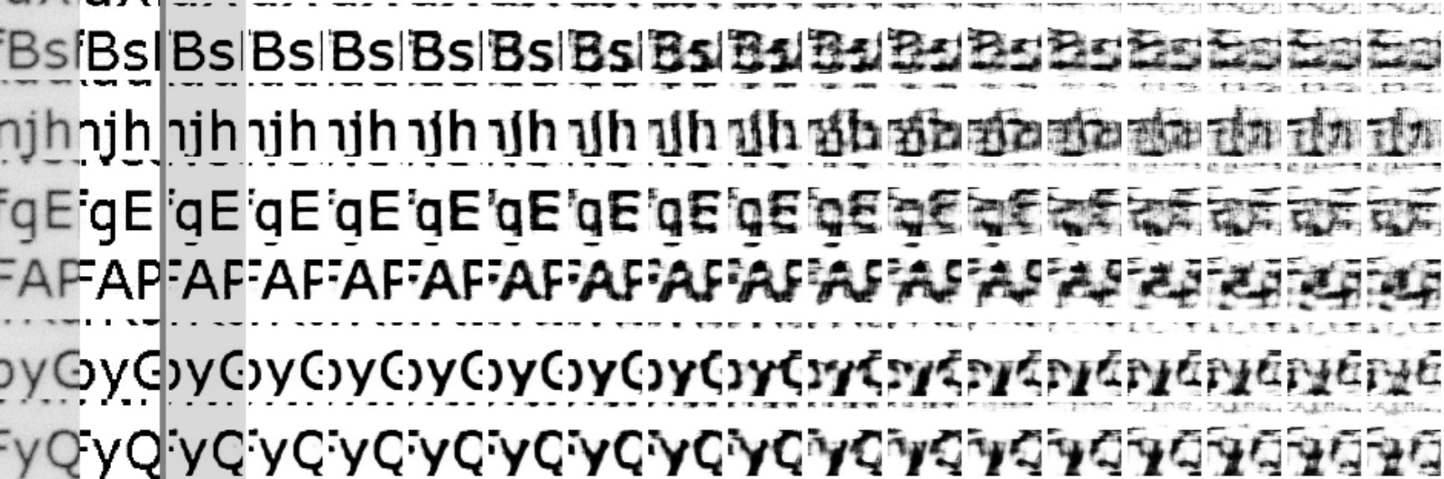
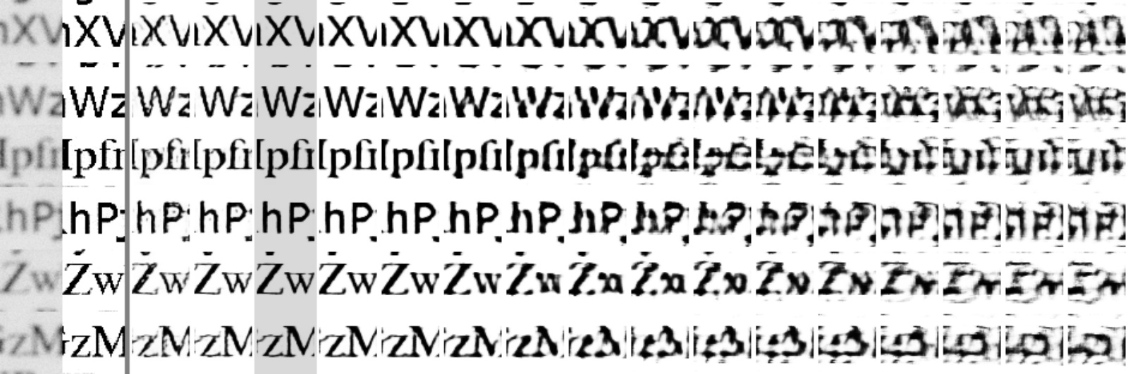
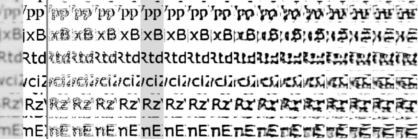
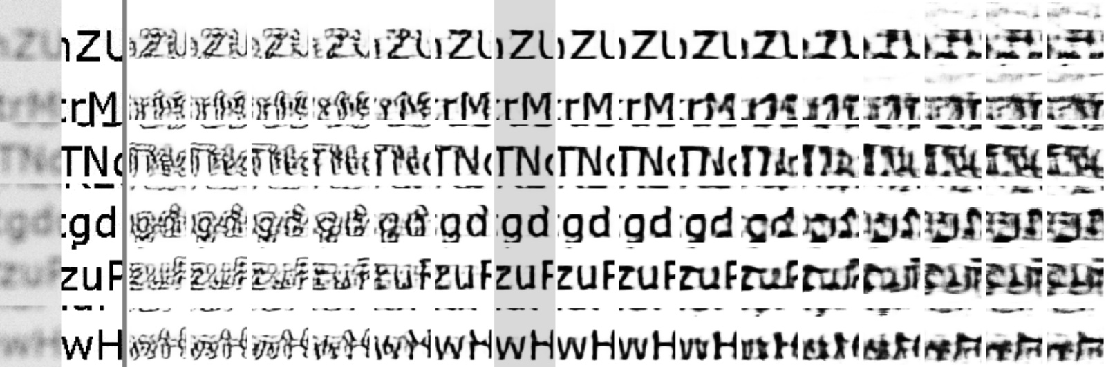
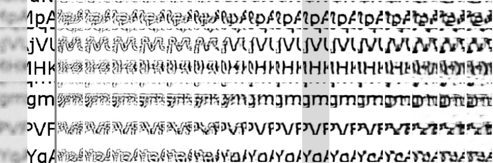
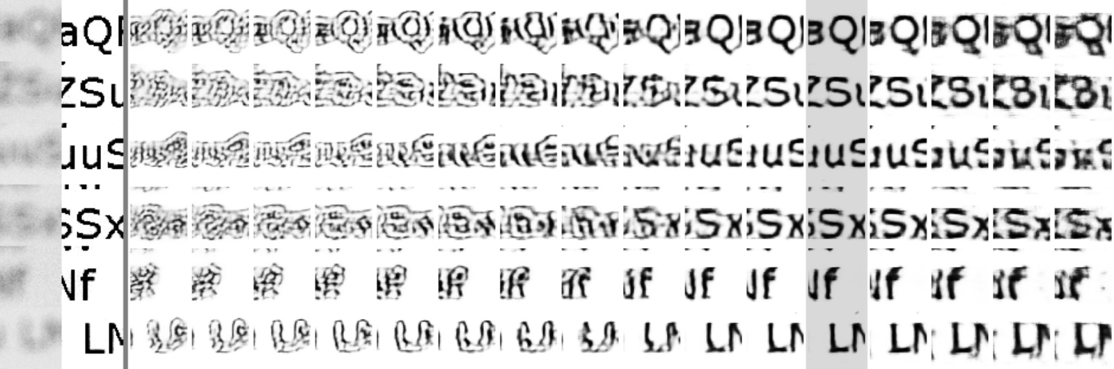
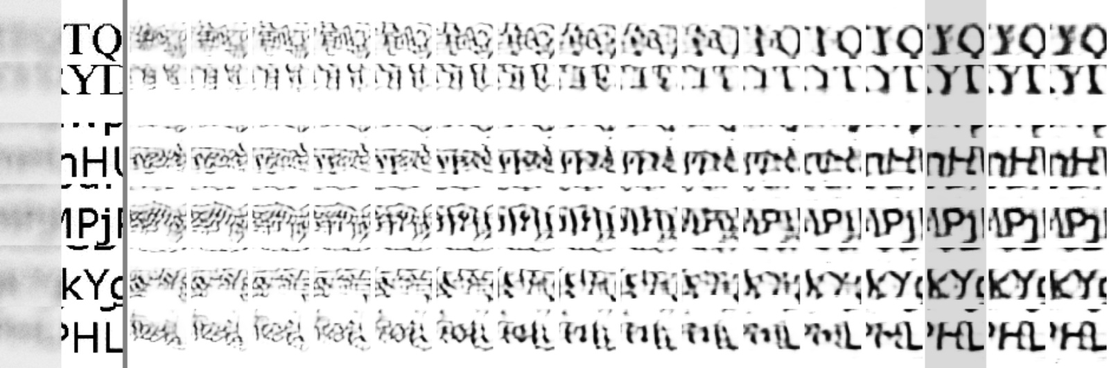
An example of the model's output is shown in Figure 8, for varying blur levels (aka,. steps). Figures 9 - 16 show how the "step" parameter affects the output. It seems very important that this parameter is set correctly. If this network was used to deblur images with an unknown blur level, the whole range would need to be tested and the best one must be picked manually, or based on some heuristic.
The contest (or "challenge") was overall very well organized, and the validation dataset came with a twist: unlike the previously released dataset which only contained alphabetical characters, the new dataset had also digits. This means that the network cannot be trained to always produce alphabetical outputs, but rather it has to be a more general algorithm. Full results can be found from the website, but in conclusion out of the 17 teams which registered to the contest, only nine submitted their final results according to the rules (on time and open sourced on GitHub). If I had entered the contest it would make ten of us, and the current (unoptimized) solution would have been at the 7th place, beating three submitted solutions. Most of the solutions could deblur images up to step 10 and more, and the top two reached amazing steps of 18 and 19 which look just plainly impossible!
Summary of the results are shown in Table 1. There is some random variation between tightly contested models, and their rank depends on which blur step is examined. At steps 4, 6 and 8 the described algorithm in this paper was ranked at places 5th, 6th and 9th from the top.
| step 4 | step 6 | step 8 | |||||||
| Team | University | stop | score | rank | score | rank | score | rank | |
| 1st | 15_A | Technische Universität Berlin, GER | 19 | 94.53 | 3 | 94.03 | 2 | 93.12 | 1 |
| 2nd | 12_B | National University of Singapore | 18 | 94.75 | 2 | 92.62 | 3 | 92.62 | 2 |
| 3rd | 01 | Leiden University, NL | 14 | 94.92 | 4 | 91.75 | 4 | 91.65 | 3 |
| 4th | 11_C | University of Bremen, GER / UK | 10 | 92.22 | 6 | 87.78 | 5 | 81.25 | 5 |
| 5th | 06 | Heinrich Heine Uni. Düsseldorf, GER | 10 | 96.40 | 1 | 94.33 | 1 | 85.92 | 4 |
| 6th | 13 | Federal University of ABC, BRA | 7 | 91.45 | 7 | 71.12 | 8 | 67.12 | 7 |
| 7th* | - | Niko Nyrhilä, FIN | 7 | 94.50 | 5 | 81.08 | 6 | 60.80 | 9 |
| 8th | 16_B | Technical University of Denmark | 6 | 90.20 | 8 | 76.45 | 7 | 68.35 | 6 |
| 9th | 04 | Dipartimento di Sciente Fisiche, ITA | 5 | 82.45 | 9 | 68.00 | 9 | 62.85 | 8 |
| 10th | 09_B | University of Campinas, BRA | 2 | 16.15 | 10 | 6.33 | 10 | 2.27 | 10 |
There remains several areas to be improved upon, some of which might result in a higher rank:
- More hyperparameter tuning, including different activation functions.
- Train the model as long as it taks, do not limit to 12 hours.
- Speed up the training by showing fewer samples of the easier blur levels, the model architecture seems to interpolate between them very well. Maybe this could be a dynamical process which happens automatically during training?
- Switch to a lower learning rate upon initial convergence, do not use the fixed 10-2.5.
- Use further blur steps for training, do not limit to steps 0 - 9. If convergence is an issue one could try to adjust sample weights so that initially the least blurred images are weighted more. More blurred images would be used mainly for fine-tuning.
- Down-scale images less than by a factor of 1 : 7, so that character details are black & white rather than grayscale.
- Include sharp images' ∂⁄∂x and ∂⁄∂y as an additional target to the network's output, maybe it would provide stronger gradients and the network would learn faster?
- Reduce overfitting by data augmentation, ideally the network would be rotation-invariant.
- Add dropout, either the standard or the 2D variant. The dropout rate is yet an other hyperparameter.
- Try regularization as well, especially the shared layer which has the most parameters.
- Current pre-processing steps aren't ideal, the model should learn not to get confused by vingetting.
- Use an other network architecture like an U-net to get local and global context, although it is closer to cheating at this point since such network was the contest winner.
But if it takes 24 hours to train the network, it will take quite a long time to find the optimal mix of even some of these options. At least it is trivial to parallelize, and consumer GPUs are still getting faster. The used GTX 1080 Ti is from 2017, so it is already 4 years old as of 2021.
Related blog posts:
|
|
|
|
|
|
|
|
|
|
