Niko's Project Corner

As I men­tioned in the pre­vi­ous ar­ti­cle about om­ni­di­rec­tional cam­eras, my Mas­ters of Sci­ence The­sis in­volved the us­age of this spe­cial kind of imag­ing sys­tem which con­sists of a tra­di­tional cam­era lens and a con­cave mir­ror, which pro­vided 360° × 90° Field of View. It was or­dered from Japan and there was some de­lay in the de­liv­ery, so mean­while I wrote an all-Mat­lab script to sim­ulate this sys­tem's prop­er­ties, cal­ibra­tion and panorama gen­er­ation in prac­tice.

The ren­der­ing ge­om­etry is based on a sin­gle in­finite ground plane, and a few dozen in­finite cylin­ders which rep­re­sent tree trunks. The whole ren­der­ing script is only 500 lines of Mat­lab code, but it has sig­nif­icant com­plex­ity be­cause of the way it uses sparse ma­trix al­ge­bra to do fast tex­ture lookups and avoid for loops, which gen­er­ally per­form badly in Mat­lab. This also makes the code au­to­mat­ically mul­ti­threaded, be­cause Mat­lab can use sev­eral cores to ex­ecute ma­trix op­er­ations.

Af­ter set­ting up the cam­era pa­ram­eters and po­si­tion, ground plane equa­tion has been de­ter­mined and tree trunks have been gen­er­ated, the script pro­ceeds to ren­der the im­age in four smaller tiles, which are later stitched to­gether. The rea­son is that oth­er­wise we might run out of mem­ory, es­pe­cially if the cal­cu­la­tions are ex­ecuted us­ing GPU prim­itives.

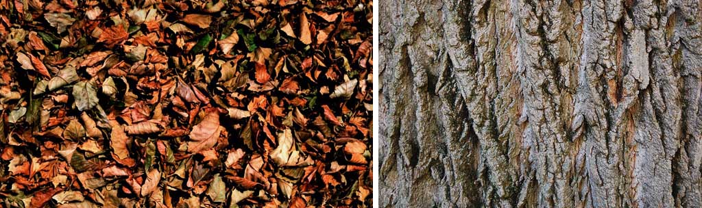
At first the light rays are casted for each im­age pixel, and their first col­li­sion with the mir­ror's paraboloid sur­face is de­ter­mined. To make the model more re­al­is­tic, also lens dis­tor­tion is sim­ulated. Af­ter the col­li­sion with the mir­ror is cal­cu­lated, the ray is re­flected based on the mir­ror's lo­cal nor­mal vec­tor. Then this orig­ina­tion point and di­rec­tion are trans­formed from cam­era's lo­cal co­or­di­nate sys­tem to world co­or­di­nates. Then their col­li­sion lo­ca­tion with the ground plane is si­mul­ta­ne­ously cal­cu­lated for all of the pix­els within the cur­rent tile, us­ing stan­dard lin­ear al­ge­bra. If the tile is 1024 × 1024 pix­els, the ma­trix A in A x = b has a size of (3 × 1024²) × (3 × 1024²) → 10¹³ elements! But since only 5 × 10^-5% of them are non-zero, solving this takes only about one second. The end result is the coordinates (3 × 1024 × 1024 elements) in which the rays hit the ground plane, which are used to sample the ground plane's texture. The used texture can be seen in Figure 1 on left. Also those pixels are ignored which would be reflected to an angle which outside the set bounds, and this produces the dark perimeter to the image. In these renderings there was no lower limit for the angle, meaning that the camera could see ''through itself'' to the ground directly under it.

Figure 1: Used tex­tures for the ground plane and tree trunks.

Next we need to it­er­ate through each tree and check it for two things. The first step is to cal­cu­late that to which pix­els this tree would be cast­ing a shadow, based on di­rec­tional light source's di­rec­tion. If this oc­curs, a rather com­plex for­mula is val­uated to de­ter­mine the amount of re­sult­ing shad­ow­ing. This takes into ac­count the trunk's di­am­eter, po­si­tions dis­tance from the trunk and any pre­vi­ously casted shad­ows. Shad­ows are drawn be­fore tree trunks, to make sure that they wouldn't in­cor­rectly shadow them. The re­sult­ing shad­ows are very con­vinc­ing, mim­ick­ing soft shad­ows' well known prop­er­ties.

At the sec­onds step we check that in which pix­els the tree trunk is vis­ible, by solv­ing the clos­est dis­tance from cylin­der's sur­face to each casted ray. Since the cylin­ders have an in­finite length, in the­ory we would see them also un­der­ground. That is why we need to con­firm that this dis­tance is smaller than the ground plane's dis­tance. If this is the case, then this dis­tance is recorded for fu­ture use.

These are the most time con­sum­ing steps, tak­ing 11 sec­onds for a tile of 1024 × 1024 pix­els when 32 trees are pre­sent. This could be op­ti­mized from the naive O(n × t) (where n is the num­ber of trees and t is the num­ber of tiles) closer to O(n), by ig­nor­ing those trees which can be de­ter­mined not to be vis­ible in the cur­rent tile, and not to cast any vis­ible shad­ows there.

Once dis­tances to trees have been cal­cu­lated, the ray-cylin­der col­li­sion lo­ca­tions are cal­cu­lated. Then the trees' sur­faces' nor­mals can be de­ter­mined, which are ran­domly per­muted to cre­ate a more re­al­is­tic re­sult. Af­ter this the re­flected ray di­rec­tions are cal­cu­lated, which are com­bined with the light source's di­rec­tion to de­ter­mine the amount of shad­ow­ing or sun ray re­flec­tion, which is ap­plied to the tree trunk tex­ture.

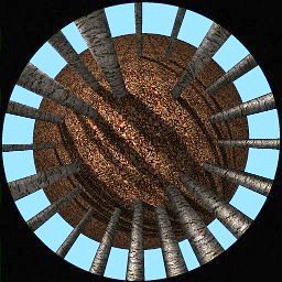
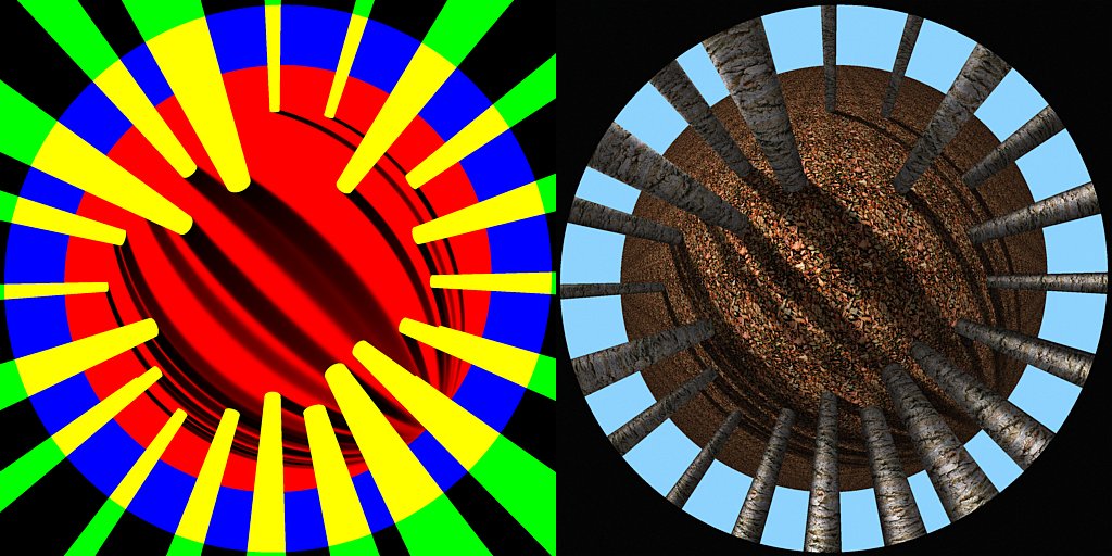
As the fi­nal step the sky is added, which is a sim­ple color re­place­ment for those pix­els which did not hit a tree and can­not see the ground plane, or which are too hor­izon­tal and see the ground plane very far away. The fi­nal out­come can be seen in Fig­ure 2. The col­ors on the left in­di­cate that which ge­om­etry af­fected each pixel's fi­nal color. Tex­tured mod­els can be seen on the right. In this case the cam­era would be look­ing up­wards, in which case the mir­ror re­flects the rays at the mid­dle of the im­age di­rectly down to­wards the ground. Rays closer to im­age bor­der are sent up­wards, and the cir­cu­lar perime­ter oc­curs from the lim­ita­tion of max­imum in­cli­na­tion an­gle to 20°. The light is orig­inat­ing from the top-left cor­ner.

Figure 2: The ren­der­ing con­sists of three steps, and their cor­re­spond­ing ob­jects are in­di­cated on the left in dif­fer­ent col­ors. The tex­tured end re­sult can be seen on the right.

Related blog posts:

Automatic map stitching, 2014 Sep (Matching: Matlab, Rendering)
Visualizing laser scanned geography, 2013 Jul (Matching: Matlab, Rendering)
Global illumination, 2013 Jul (Matching: Rendering)
CUDA realtime rendering engine, 2013 Jul (Matching: Rendering)
Simulating gravitational field near a torus, 2016 Apr (Matching: Matlab)