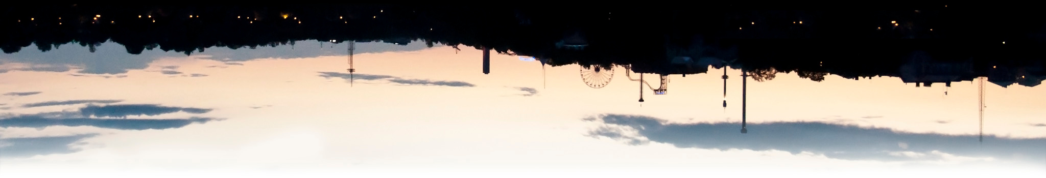

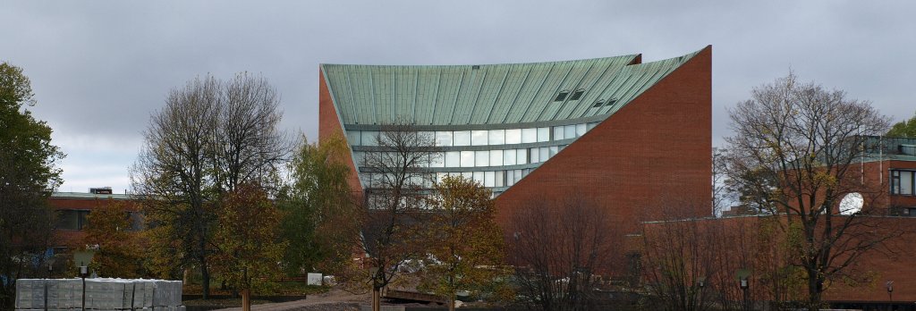
During the summer of 2012 when I was mainly working on my Master's Thesis, I also had a look at National Land Survey of Finland's open data download service. There I downloaded a point cloud dataset which had typically 4 - 5 measured points / square meter. This means that to visualize a region of 2.5 × 2 km, I had to work with a point cloud consisting of 5 × 2500 × 2000 → 25 million points. I chose to concentrate on my campus area, because I know it well and it has many interesting landmarks. For example the iconic main building can be seen in Figure 1.
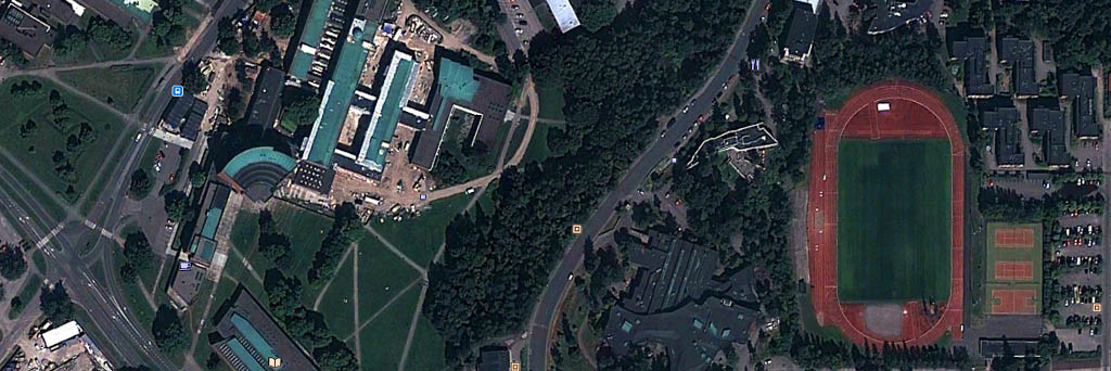
From the satellite view at Figure 2, we can identify numerous landmarks and regions such as the main building on the left, sports center on the right and lots of trees and smaller buildings. At the time of taking these images there was also an ongoing construction project.
At first I just loaded the whole point cloud of the region into Matlab, but I quickly realized that the naive approach would be too slow. Thus I decided to pre-process the data in C++, and use Matlab only for the final visualization step. In C++ I inserted all points into a quadtree data structure, to enable efficient range queries. Only the longitude and latitude were used, because the height is irrelevant in this scenario.
Once the data structure was constructed, it is used to sample the point clouds on a regular grid. In this case I created a dataset 2500 × 2000 meters, where it was sampled at one meter intervals. For each sample point the data points within a radius of 1.5 meters were queried. From these the minimum and maximum height were determined, and also the average height using a Gaussian kernel for weighting. These results were stored into a txt file, which was then read in by Matlab.
In Matlab's output the pixel's brightness corresponds to the mean height, but there are two additional coloring rules. On the regions which contained trees, some of the laser rays hit trees' top, and some hit the ground level. By observing the height difference in lowest and highest recorded point, it can be estimated whether there was a tree nearby. Identified trees are encoded in green (using YCbCR colorspace).
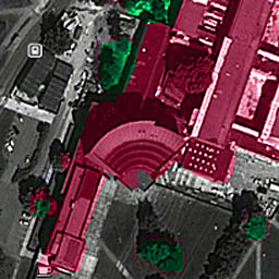
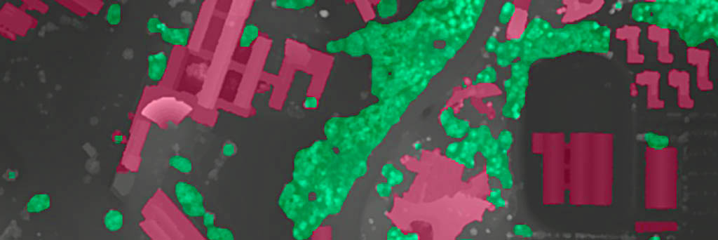
An other heuristics was to identify walls of the buildings, by setting a criteria that they are at least 1.5 meters above the local ground level. Then these enclosed areas are identified as buildings, and are color coded as red in the final image, which can be seen in Figure 3. The height profile of the main building is clearly visible, and most of the buildings and trees are correctly identified.
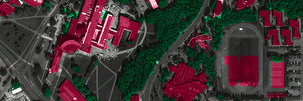
The rendered output is compared against the satellite view, by using the satellite image for grayscale information and the laser data's classification as color channels. As can be seen from Figure 4, there is a very good agreement between these two independent data sources. The only main differences are one mis-classified at the bottom right, and the large structure that was at the sports center at the time when laser scanning took place. Most of the trees are correctly identified as well.
Related blog posts:
|
|
|
|
|
|
|
|
|
|
