Niko's Project Corner

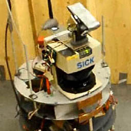
At spring 2012 I did a course in robotics, which in­volved pro­gram­ming a semi-au­to­matic robot which could fetch items from pre-de­ter­mined lo­ca­tions and re­turn them back to cor­rect de­posit bins. I had a team of four peo­ple, and I solved the prob­lems of con­tin­uous ro­bust robot lo­cal­iza­tion, task plan­ning and path plan­ning. Oth­ers fo­cused on the over­all source code ar­chi­tec­ture, state-ma­chine logic, closed loop driv­ing con­trol and other gen­eral top­ics. The used robot can be seen in Fig­ure 1.

Figure 1: The used robot with two-wheel se­tup which en­ables it to ro­tate in-place. It has 2D laser scan­ner, odom­etry and we­bcam sen­sors.

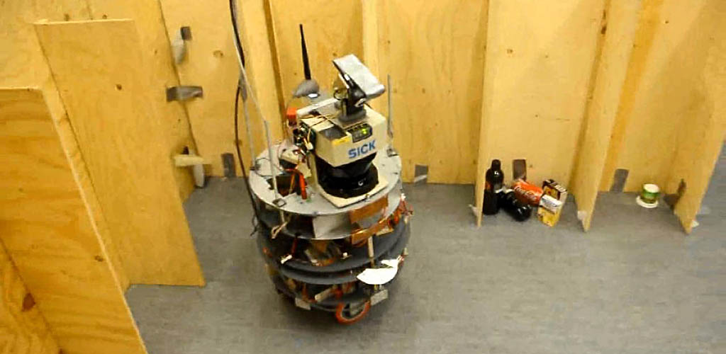
The ini­tial path plan­ning is done by uti­liz­ing a pre-drawn bitmap, in which each pixel cor­re­sponds to 2 cm in real life. This map rep­re­sents the al­lowed po­si­tions in which the robot is al­lowed to move, and ex­tra padding is added to ac­count for robot's phys­ical size. A few of these maps can be seen in Fig­ure 2. Us­ing this dis­crete map pre­sen­ta­tion it is fairly straight for­ward to find the short­est path by us­ing for ex­am­ple A* search. But in prac­tice the short­est path might not be the fastest to drive through, es­pe­cially when the path has tight turns. Also it doesn't take the robot's fi­nal head­ing into con­sid­er­ation.

Figure 2: Two maps which also dis­play the planned paths with smooth curves and the head­ing op­ti­miza­tion. The path on the right makes the robot to ar­rive to the end point in the de­sired ori­en­ta­tion, which wouldn't be the case if the short­est path was used. Ma­genta points are laser mea­sure­ments be­ing pro­jected to the map over­lay, based on the es­ti­mated robot's po­si­tion and head­ing.

To im­prove the path, a gra­di­ent de­scent al­go­rithm is used to min­imize a bet­ter cost func­tion. The to­tal cost of the path is the weighted sum of its length, cur­va­ture and the fi­nal head­ing er­ror. The start­ing and end­ing lo­ca­tions can­not be changed, but all other way points are free to to be ad­justed. The gra­di­ent de­scend it­er­ation starts by nu­mer­ically es­ti­mat­ing ^∂⁄_∂pi f(p_1, p_2, ..., p_n), where i = 2, ..., n-1, and p_i is the location of the i^th way point. However this parametrization isn't ideal for the optimization process.

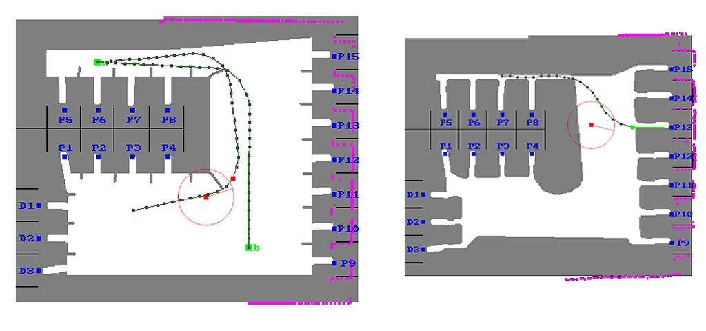
To make it eas­ier to im­ple­ment the op­ti­miza­tion al­go­rithm, each way point's ad­just­ment is parametrized by a sin­gle scalar, which in­di­cates the way point's off­set from its cur­rent lo­ca­tion, or­thog­onal to the path's cur­rent di­rec­tion. This is il­lus­trated in Fig­ure 3. Once each of the par­tial deriva­tives ^∂⁄_∂lif(p_1, p₂ + l₂ n₂ , ..., p_n) are calculated, the descend step can be performed towards the direction in which the cost function decreases the fastest. Some extra logic is needed to determine the step length and a suitable stopping criteria. Also it must be ensured that the refined path does not go through a forbidden region in the map. The optimized path is a lot faster to drive through than the shortest path, because the robot can drive broader arcs at higher speeds, and reach the end point at already correct heading.

Figure 3: The orig­inal path from path find­ing is shown in blue, and the op­ti­mized path is shown in red. Short red lines in­di­cate the cur­rent or­thog­onal di­rec­tion, which is used at the gra­di­ent de­scend op­ti­miza­tion pro­cess.

The im­ple­mented lo­cal­iza­tion al­go­rithm is quite in­ter­est­ing as well. The robot has a ro­ta­tory en­coder for both wheels, so we have odom­etry data avail­able. How­ever it ac­cu­mu­lates er­rors quite fast, and also the robot's ini­tial po­si­tion should be known. In ad­di­tion it can­not re­cover from the robot be­ing man­ually moved. This is why it is bet­ter to uti­lize the laser scan­ner's mea­sure­ment data, which is the dis­tance mea­sure­ment from ±90°, re­turn­ing 181 read­ings in to­tal, with an ac­cu­racy of a few cen­time­tres.

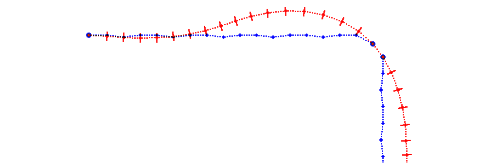
The most ad­vanced so­lu­tion would be to im­ple­ment a SLAM (Si­mul­ta­ne­ous Lo­cal­iza­tion And Map­ping) al­go­rithm, which can build a map of the un­known re­gion on-the-fly, while us­ing the same map to do lo­cal­iza­tion. To make the al­go­rithm ro­bust, it should im­ple­ment fea­tures such as loop clos­ing and fil­ter er­ro­neous data. In our pro­ject the en­vi­ron­ment was static and known in ad­vance, so I de­cided to base the lo­cal­iza­tion al­go­rithm on known land­marks such as cor­ners and walls. These are rel­atively easy to be ro­bustly de­tected from laser read­ings, and an ex­am­ple read­ing is shown in Fig­ure 4. An other al­ter­na­tive ap­proach would have been to use a par­ti­cle fil­ter or Kalman fil­ter, but these are non-triv­ial to im­ple­ment and de­bug, to make sure you'll never re­port an in­cor­rect lo­ca­tion.

Figure 4: Land­marks (cor­ners and walls) are de­tected from the laser data (on the left), and it is matched with the pre-de­fined map. The lo­ca­tion and ori­en­ta­tion with most votes is in­di­cated by the green line.

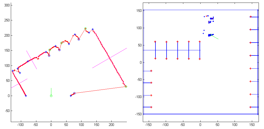
The ac­tual lo­cal­iza­tion al­go­rithm works by us­ing groups of a few land­marks, and try­ing to find a sim­ilar con­fig­ura­tion from the map. For ex­am­ple one cor­ner is not enough to de­ter­mine the lo­ca­tion, but two cor­ners is al­ready suf­fi­cient, if we knew that which two cor­ners of the map those cor­ners match to. Sim­ilarly a sin­gle point and a wall are suf­fi­cient for this pur­pose. The al­go­rithm makes hy­pothe­ses about these cor­re­spon­dences, and if the re­sult­ing lo­ca­tion and ori­en­ta­tion is some­what con­sis­tent with the laser read­ings (for ex­am­ple no walls are ob­served at the known empty re­gions of the map), a vote is casted for this can­di­date lo­ca­tion. Clus­ters of these votes can be seen on the right of Fig­ure 4. The clus­ter with most votes is then de­ter­mined, and that is the fi­nal lo­ca­tion es­ti­mate.

The robot can­not rely only on the laser based lo­cal­iza­tion, be­cause the robot might be fac­ing a wall, in which case there might not be suf­fi­cient land­marks avail­able for un­am­bigu­ous lo­cal­iza­tion. It is cru­cial that the robot knows its po­si­tion at all times, be­cause that is an in­te­gral part of the closed loop con­trol logic which de­ter­mi­nes the con­trol sig­nals for the wheels, to drive the robot along a planned path. To over­come this prob­lem, I de­cided to al­ways rely on the odom­etry based po­si­tion es­ti­mate in­stead.

When the robot is mov­ing and the laser based lo­cal­iza­tion has been suc­cess­ful for the past one me­ter or so, ac­cu­mu­lated er­rors in the odom­etry can be fully com­pen­sated for. So in prac­tice the in­cor­rect odom­etry es­ti­mate is trans­formed into cor­rect world co­or­di­nates, and this map­ping is re-cal­ibrated al­ways when pos­si­ble. This com­bined al­go­rithm has ben­efits of both sen­sor sys­tems, and works re­li­ably in all sce­nar­ios. If the robot is moved or the sys­tem is re-started, the cal­ibra­tion is done by just driv­ing a few me­ters.

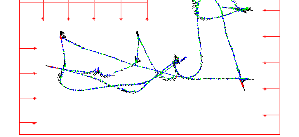
Ex­am­ple re­sults of this al­go­rithm are shown in Fig­ure 5. The robot was driven around by us­ing man­ual con­trol, and the data was logged into a file. Later this file was read by a C++ pro­gram, which ex­ecutes the lo­cal­iza­tion al­go­rithm and prints out the out­put into a file. Then this file was read into Mat­lab, in which the es­ti­mated path was plot­ted. Red dots on the path in­di­cate lo­ca­tions in which the laser data could not be used to un­am­bigu­ously de­ter­mine the lo­ca­tion. It is also seen that the lo­ca­tion es­ti­mates don't jump around, and in­stead the drawn paths are very smooth. This is due to us­ing the odom­etry based lo­ca­tion as a start­ing point, and us­ing the laser based lo­ca­tion only for cor­rect­ing odom­etry's er­rors.

Figure 5: The robot's path is re­con­structed from the logged sen­sor read­ings.

Related blog posts:

Very fuzzy searching with CUDA, 2015 Nov (Matching: C++)
Efficient in-memory analytical database, 2013 Dec (Matching: C++)
Real-time Heat Map Generator, 2013 Nov (Matching: C++)
HTTP API load tester, 2013 Nov (Matching: C++)
Real-time interest point tracking, 2013 Jul (Matching: C++)