Niko's Project Corner

I wanted a real-time map gen­er­ator to vi­su­al­ize re­gional prop­erty price changes based on cho­sen time in­ter­val. I didn't want to re­sort to pre-gen­er­ated tiles, be­cause this would pre­vent user-cus­tomized out­put and limit con­fig­ura­tion op­tions. To get the best per­for­mance, I im­ple­mented a FastCGI pro­cess in C++ with a REST­ful in­ter­face to gen­er­ate the re­quired tiles in par­al­lel. The re­sult­ing pro­gram can gen­er­ate a cus­tomized 1280 × 720 res­olu­tion JPG in 30 mil­lisec­onds and equiv­alent PNG in 60 mil­lisec­onds.

Heat maps are great way to vi­su­al­ize scalar fields (such as sur­face tem­per­ature, pop­ula­tion den­sity or prop­erty prices). Un­for­tu­nately on­line maps are usu­ally based on pre-gen­er­ated tiles, and thus don't al­low more user-cus­tomized func­tion­al­ity. An other in­ter­est­ing ap­proach is to first load pre-gen­er­ated map tiles and then use HTML5 and JavaScript to draw a semi-trans­par­ent color layer on top. This might be the tech­ni­cally most ad­vanced ap­proach, but it re­lies heav­ily on client-side cal­cu­la­tions and it might not be well sup­ported in older browsers or in­side mo­bile ap­pli­ca­tions. It might also force the send­ing sen­si­tive or pro­pri­etary in­for­ma­tion to the browser, which would be a great in­ter­est of com­peti­tors.

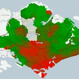
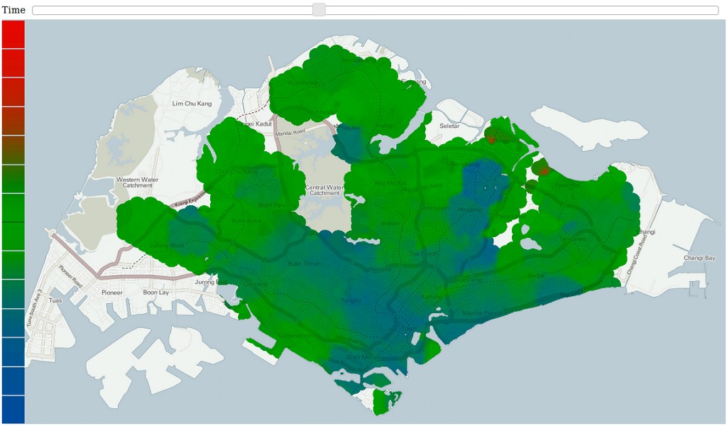
To avoid these is­sues, I wrote all gen­er­ation logic on the server side in C++, and it is ac­ces­si­ble via HTTP by us­ing Ng­inx (or any other HTTP server) and FastCGI com­mu­ni­ca­tion with the im­age gen­er­ation pro­cess. The tech­nique de­scribed here ap­plies to var­ious sce­nar­ios, but when I first wrote this I wanted to vi­su­al­ize pro­pri­etary re­gional prop­erty price in­dexes which I de­vel­oped for Prop­er­tyGuru.com.sg. I also in­cluded a slider to choose the time pe­riod for which the quar­terly price in­dex change is cal­cu­lated. The proof-of-con­sept UI and the map out­put can be seen in Fig­ure 1. Green col­ors in­di­cate a price in­dex change of ±2%, red col­ors are up-to +15% and blue col­ors are for -15%.

Figure 1: Ex­am­ple UI with the time axis slider and the re­sult­ing map. This shows how prop­erty prices started to de­crease in cen­tral Sin­ga­pore at 2008 mid­point, af­ter they peaked at early 2008.

In this case re­gional price in­dexes were cal­cu­lated at 330 me­ter in­ter­vals form­ing a hexag­onal grid, which to­tals in ap­prox­imately 2000 pre-cal­cu­lated in­dexes. When the pro­cess is spawned it first reads in this price in­dex data, to­gether with the back­ground map file, mask for land/wa­ter clas­si­fi­ca­tion and a con­fig­ura­tion file to con­vert pixel co­or­di­nates into lat­itude and lon­gi­tude and back. To op­ti­mize the code for map gen­er­ation speed, each pixel's lo­ca­tion is pre-pro­cessed to check if it is in wa­ter. If it is not, then its near­est three price in­dexes are de­ter­mined and stored for fu­ture use. The fi­nal out­put is a weighted av­er­age of the near­est price in­dexes, the weight be­ing roughly in­versely pro­por­tional to the squared dis­tance from the pixel. These weights are stored along side with point­ers to near­est price in­dexes.

In ad­di­tion to price in­dex data, also the un­der­ly­ing map and the wa­ter mask is pre-loaded in mem­ory and split into 2 × 4 sub-im­ages. These are later used to gen­er­ate and store eight tiles in par­al­lel. At the de­fault res­olu­tion of 1280 × 720 each sub-im­age has the res­olu­tion of 320 × 360 pix­els.

Each re­quest to the API in­cludes the start and end date of the time pe­riod for which price in­dex changes are cal­cu­lated. Price in­dexes are tra­versed in eight par­al­lel threads, and the price in­dex's change be­tween the two points in time are stored within its own class mem­ber. This avoids the price in­dex change be­ing cal­cu­lated for each pixel sep­arately, and in­stead it can be shared by any num­ber of pix­els.

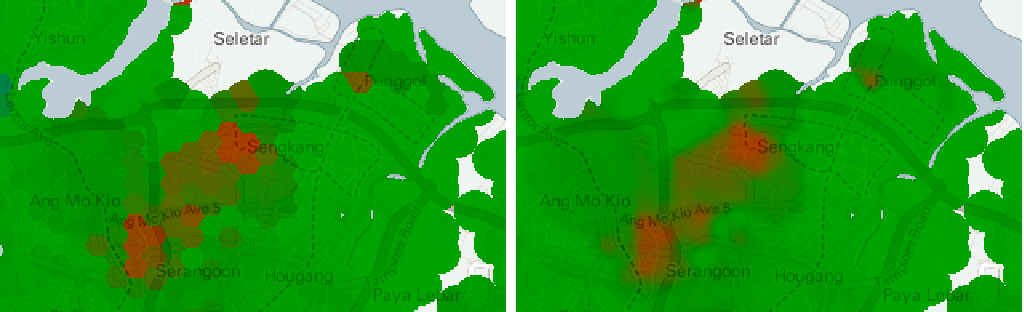
Af­ter price in­dex changes are com­puted, each sub-im­age is ren­dered in par­al­lel. Within each sub-im­age each pixel is tra­versed, and if it con­tains point­ers to near­est price in­dexes their weighted av­er­age value is cal­cu­lated. This value is con­verted to RGB color from YCbCr color space and al­pha-blended to the un­der­ly­ing map im­age. The value in­ter­po­la­tion is very im­por­tant to avoid block­ing be­tween cell bound­aries, as can be seen from Fig­ure 2.

Figure 2: This en­larged com­par­ison shows the im­por­tance of in­ter­po­lat­ing the value from three near­est price in­dex lo­ca­tions. Oth­er­wise the un­der­ly­ing grid's struc­ture is clearly vis­ible in color tran­si­tions.

When sub-im­ages are ready, they need to be com­pressed into a stan­dard im­age for­mat such as JPEG or PNG. Since al­pha-blend­ing has al­ready been done, there is no prob­lem us­ing the JPEG for­mat to pro­duce smaller im­age files. It is also a lot faster for­mat to com­press to, but it will in­tro­duce com­pres­sion ar­ti­facts. PNG on the other hand is loss-less and sup­ports the al­pha chan­nel, so it has its ben­efits. Also the com­pressed im­ages could be tem­porar­ily be stored in-mem­ory and dis­carded soon af­ter, or stored into a more per­ma­nent cache folder in the file sys­tem. To keep my code sim­ple I only im­ple­mented the file sys­tem based so­lu­tion, and then I can also let Ng­inx to han­dle this static con­tent.

When the browser makes the GET re­quest to in­di­cate which time span's im­ages it wishes to re­ceive, all the steps above are ex­ecuted. Once this is done, the browser re­ceives a JSON re­sponse which lists URLs of the eight gen­er­ated sub-im­ages. Then it only needs to it­er­ate through this list and up­date the URLs of the UI im­age tile el­ements. The whole im­age gen­er­ation pro­cess for 1280 × 720 out­put takes only 60 mil­lisec­onds in PNG for­mat and 30 mil­lisec­onds in JPEG for­mat, so clearly the real-time con­strains are well met. These tim­ings are from an Ubuntu run­ning in­side a vir­tual ma­chine with six avail­able cores. It seems that the only bot­tle­neck is the net­work over which the im­ages are trans­ferred.

Related blog posts:

Efficient in-memory analytical database, 2013 Dec (Matching: C++, FastCGI)
HTTP API load tester, 2013 Nov (Matching: C++, FastCGI)
Very fuzzy searching with CUDA, 2015 Nov (Matching: C++)
Real-time interest point tracking, 2013 Jul (Matching: C++)
Global illumination, 2013 Jul (Matching: C++)