Niko's Project Corner

The NYC taxi­cab dataset has seen lots of love from many data sci­en­tists such as Todd W. Schei­der and Mark Litwintschik. I de­cided to give it a go while learn­ing Clo­jure, as I sus­pected that it might be a good lan­guage for ETL jobs. This ar­ti­cle de­scribes how I loaded the dataset, nor­mal­ized its con­ven­tions and columns, con­verted from CSV to JSON and stored them to Elas­tic­search.

My older desk­top (let's call it "Ma­chine A") has In­tel i5 3570K (quad-core with­out hy­per-thread­ing), 24 GB RAM and 2 x 250 GB Sam­sung 840 EVOs for data. The newer ("Macine B") has In­tel i7 6700K (quad-core with hy­per-thread­ing), 64 GB RAM and 2 x 500 GB Sam­sung 750 EVOs for data. Based on CPU bench­marks it should be about twice as fast as the i5, be­ing roughly equiv­alent 40 AWS ECUs.

One main goal was to get doc­uments in­dexed to Elas­tic­search as fast as pos­si­ble. Thus I used two SSDs RAID-0 type con­fig­ura­tion by us­ing ZFS on Linux. The first ma­jor ob­sta­cle was that at ini­tially I got great write per­for­mance but af­ter 10 min­utes or so it had dropped to only 40 MB/s! Based on cur­rent and past is­sues at its Github repo ZoL doesn't seem pro­duc­tion ready yet, but I man­aged to find a workaround for my case. When I for­mat­ted SSDs to EXT4 and cre­ated a 450 GB empty files there, I could suc­cess­fully cre­ate a ZFS pool out of them it could sus­tain the ex­pected IO per­for­mance. This was a quite puz­zling sit­ua­tion, but I ended up cre­at­ing a 8 GB file to EXT4-for­mat­ted Sam­sung 850 EVO m2 card (which is the main sys­tem disk) and us­ing it as ZIL for my pool. For some rea­son this kept the IO per­for­mance at nor­mal lev­els and I did not have to run ZFS on top of EXT4.

CSV files are stored in a Gzipped for­mat, from which they are lazily read as Clo­jure strings by java.util.zip.GZIP­In­put­Stream. Ini­tial im­ple­men­ta­tion would slurp the whole CSV string and pass it to read-csv, but this at too much RAM when mul­ti­ple large files are be­ing pro­cessed in par­al­lel. The pro­cess of con­vert­ing CSV rows in to Elas­tic­search doc­uments is quite straight-for­ward. The code has a lookup dic­tio­nary to map CSV columns into JSON fields of speci­fic types. In to­tal there are 36 fields. Yel­low and Green taxi­cab datasets had some dif­fer­ences on column nam­ing but at least their mean­ing was easy to rec­og­nize. The code also gen­er­ates some new fields to each doc, such as the time of day when the trip started (0 - 24 h), how many kilo­me­ters were trav­elled lat­itude / lon­gi­tude wise and what was the av­er­age speed dur­ing the trip. It also stores that day's weather at Cen­tral Park to each doc­ument, as Elas­tic­search does not have ad-hoc joins un­like SQL databases.

Orig­inally I gen­er­ated doc­ument ids in Clo­jure and used those to skip chunks which had al­ready been in­serted to ES, which was handy when I was it­er­at­ing the code and sort­ing out mal­formed data. Later I dis­carded this as it slows down in­dex­ing pro­cess quite a lot. Nev­er­the­less doc id gen­er­ation code was still used it to fil­ter out du­pli­cates be­fore sendin them to ES. But there are less than hun­dred of them so now I don't even bother re­mov­ing them. It was caus­ing quite a lot of mem­ory and garbage col­lec­tion over­head for very lit­tle gain, but I'm sure du­pli­cate re­moval util­ity will be use­ful on other pro­jects.

There are many fac­tors which af­fect in­dex­ing per­for­mance, and I didn't care­fully mea­sure all of their im­pacts as it is quite te­dious to ex­ecute and your mileage will vary any­way. Note that many ar­ti­cles on the topic Elas­tic­search op­ti­miza­tions are for ver­sions of 1.x and 2.x but aren't rel­evant on lat­est ES 5.x ver­sions. CSV pars­ing is sin­gle-threaded, so to uti­lize mul­ti­ple CPU cores many files are parsed in par­al­lel. At first I used my own code for this, based on Clo­jure's pmap but with con­fig­urable num­ber of threads. How­ever seemed to work poorly when some files took much longer to pro­cess than oth­ers, and par­al­lelism di­min­ished un­til the larger file was fin­ished and then new fu­tures were deref­er­enced. This was re­solved by us­ing Clay­poole's mag­nif­icent up­for, which will ex­ecute the jobs in N par­al­lel threads and re­turn the fastest re­sults first. Doc­uments were bulk-up­loaded in chunks of 1000.

I had one in­dex / year / com­pany, and each in­dex had only ten shards. I started with only one shard / in­dex but it caused merge throt­tling in the long run as in­dexes grow to tens of gi­ga­bytes. For ex­am­ple the in­dex taxi­cab-yel­low-2014 has 164.2 mil­lion docs and takes 48.5 GB of stor­age.

In­dex­ing from A to B was con­strained by A's CPU power to trans­form CSV rows to JSON, in­dex­ing them to Elas­tic­search over a gi­ga­bit LAN at 100 - 150 Mbit/s. Ma­chine B's CPU us­age was fluc­tu­at­ing be­tween 30 and 50 per­cent. In 10 min­utes it could in­dex 9.55 mil­lion doc­uments, thus av­er­ag­ing at 15931 docs / sec­ond. When us­ing only ma­chine B to han­dle both work­loads it would be sat­urated by CPU, to­tal­ing at 11.9 mil­lion docs in 10 min­utes, or 19869 docs / sec­ond. When in­dex­ing from ma­chine B to ma­chine A it wasn't clear where the bot­tle­neck was as both CPUs were used at 50 per­cent. It could be caused by buggy firmware on my 840 EVOs as I haven't up­dated them yet. Any­way, this se­tup man­aged to store only 4.6 mil­lion docs in 10 min­utes, or av­er­ag­ing at 7746 docs / sec­ond. Top per­for­mance was ob­tained by pars­ing CSVs on both ma­chi­nes and host­ing ES on ma­chine B, to­tal­ing at 14.3 mil­lion docs, or at av­er­age of 23909 docs / sec­ond. Even at this speed in­dex­ing 1 bil­lion doc­uments would take about 11.6 hours.

In the end I used just ma­chine B to in­dex all doc­uments in a sin­gle go, which took 910 min­utes and stored 942.1 mil­lion doc­uments. Then I "force merged" in­dexes to have at most 8 seg­ments each, this took 44 min­utes. Fi­nally merg­ing them down to 1 seg­ment took 302 min­utes, al­though CPU and disk IO us­age was very low. It seems to have build-in throt­tling as well, but I couldn't find de­tailed doc­umen­ta­tion. The fi­nal size on disk was 309 GB.

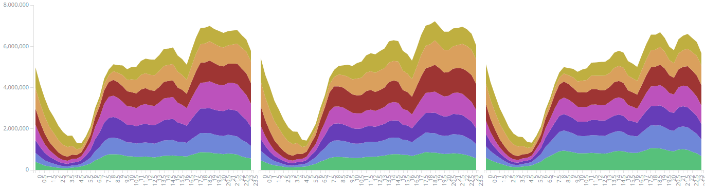
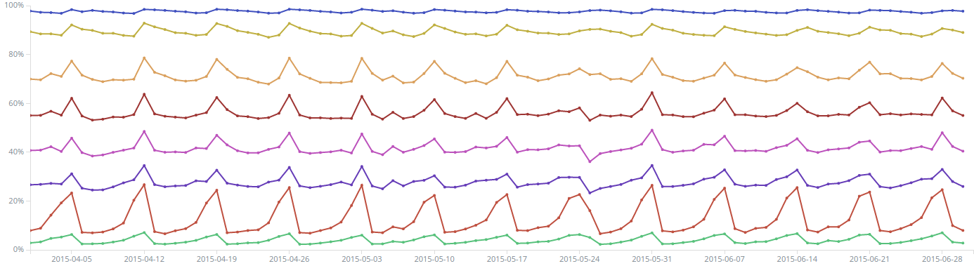
Once the data is stored to ES there are end­less pos­si­bil­ities for in­ter­est­ing anal­ysis. Kibana makes it easy to get started with un­der­stand­ing the dataset and ex­ecut­ing ad-hoc queries, but of course if you want full con­trol over de­tails and op­ti­miza­tions then you'll have to im­ple­ment lots of stuff your­self. Here I'll just show pat­terns from a sin­gle fact: the date-time when the trip started. This is split into three parts: date, day of week and time of day. One can ex­pect week­ends hav­ing dif­fer­ent taxi de­mand than rest of the days.

Figure 1: Monthly num­ber of rides on dif­fer­ent week days day and time of day.

Figure 2: Monthly share of rides on dif­fer­ent week days and time of day.

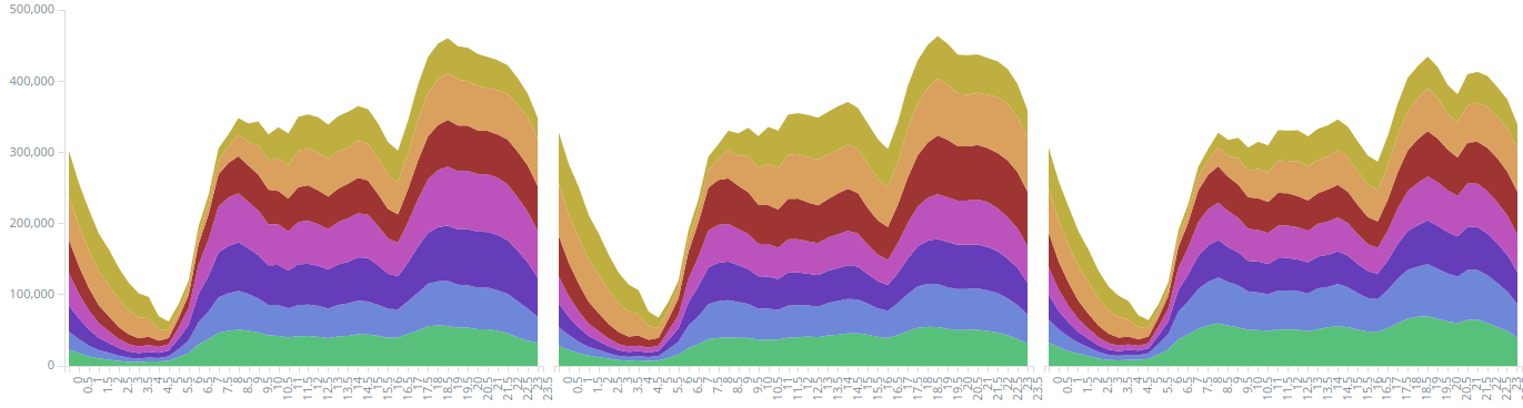
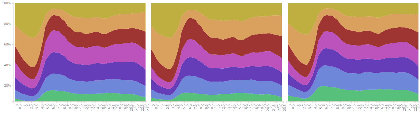
All these statis­tics were cal­cu­lated from data from 2015-04-01 to 2015-06-30, which is a to­tal of 43.3 mil­lion trips. The first set of fig­ures 1 to 3 uses Kibana's Area chart, which sup­ports many use­ful fea­tures such as split­ting ar­eas by sub-ag­gre­ga­tion and show­ing per­cent­ages in­stead of to­tals.

Figure 3: Monthly amount of spent dol­lars to taxi rides on dif­fer­ent times of day and time of day.

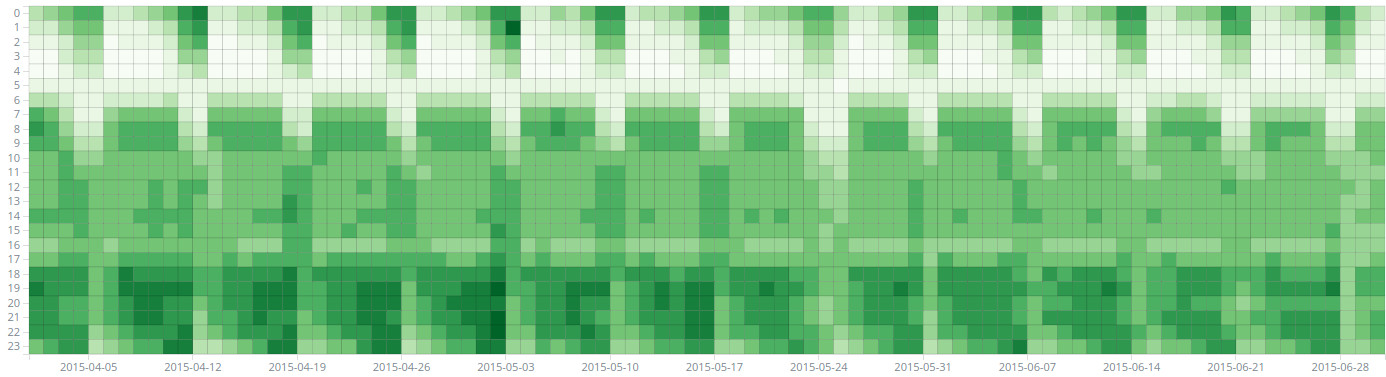
An other in­ter­est­ing vi­su­al­iza­tion is the Heatmap chart, which is seen on Fig­ure 4. It lets you choose how doc­uments are "buck­etet" along the x and y axis and what is the vi­su­al­ized met­ric. This makes weekly cy­cles quite vis­ible es­pe­cially in 2 - 5 am range but I find it more dif­fi­cult to ex­trap­olate the data for­ward when com­pared to line charts. It doesn't han­dle out­liers nicely, at least if the his­togram ag­gre­ga­tion is used. Luck­ily they are easy to fil­ter out in the query phase, if the ex­pected data range is known.

Figure 4: Heatmap on num­ber of taxi trip at dif­fer­ent week days and times of day.

The fi­nal ex­am­ple uses Line chart and per­cen­tile ranks ag­gre­ga­tion. It cal­cu­lates for each day that how many per­cent of that day's trips have oc­curred be­fore a speci­fic time of day, for ex­am­ple 6 am. Also this graph shows the ma­jor ef­fect of week­ends is on taxi trip fre­quency be­tween 1 and 6 am.

Figure 5: Per­centile ranks of trips at 1, 6, 10, 13, 16, 19, 22, and 23.5 hours.

Related blog posts:

Benchmarking Elasticsearch and MS SQL on NYC Taxis, 2017 May (Matching: Clojure, Databases, Elasticsearch, GitHub)
An efficient schema for hierarchical data on Elasticsearch, 2016 Nov (Matching: Business Intelligence, Databases, Elasticsearch)
Very fuzzy searching with Elasticsearch, 2015 Oct (Matching: Databases, Elasticsearch, GitHub)
Mustache templates in Clojure, 2017 Jan (Matching: Clojure, GitHub, JVM)
English hyphenation algorithm in Clojure, 2016 Aug (Matching: Clojure, GitHub, JVM)