Niko's Project Corner

The NYC Taxi dataset has been used on quite many bench­marks (for ex­am­ple by Mark Litwintschik), per­haps be­cause it has a quite rich set of columns but their mean­ing is mostly triv­ial to un­der­stand. I de­vel­oped a Clo­jure pro­ject which gen­er­ates Elas­tic­search and SQL queries with three dif­fer­ent tem­plates for fil­ters and four dif­fer­ent tem­plates of ag­gre­ga­tions. This should give a de­cent in­di­ca­tion of these databases per­for­mance un­der a typ­ical work­load, al­though this test did not run queries con­cur­rently and it does not mix dif­fer­ent query types when the bench­mark is run­ning. How­ever bench­marks are al­ways tricky to de­sign and ex­ecute prop­erly so I'm sure there is room for im­prove­ments. In this pro­ject the tested database en­gi­nes were Elas­tic­search 5.2.2 (with Or­acle JVM 1.8.0_121) and MS SQL Server 2014.

The first fil­ter com­bi­nes a ran­dom range query on a 14-days long in­ter­val be­tween 2013-01-01 and 2016-12-01 with a ran­domly po­si­tioned 2 x 2 km bound­ing box on the pickup po­si­tion. Nat­urally this re­sults in a ran­dom num­ber of match­ing trips, but this is taken into ac­count by plot­ting query times against the num­ber of match­ing rows. 25th, 50th and 75th per­centiles on the num­ber of match­ing trips for this fil­ter were about 50, 7k and 100k. This high dy­namic range asks for log-log plots for vi­su­al­iza­tion.

The sec­ond type of fil­ter con­sists of three parts. The first one is a ran­dom 60-day long in­ter­val be­tween 2013-01-01 and 2016-10-01. Sec­ond cri­te­rion is the amount of paid tip, hav­ing the start­ing value rang­ing from 0 to 15 dol­lars and the in­ter­val length was 2 dol­lars. The third cri­te­rion was the day of week, in­di­cated by an in­te­ger be­tween 1 and 7. The 25th, 50th and 75th per­centiles were 9k, 38k and 232k.

The last type of fil­ter com­bi­nes a range query on the travel du­ra­tion in hours start­ing from 0 - 3 hours and hav­ing the length of 15 min­utes with a terms query on the ex­act num­ber of pas­sen­gers (ran­dom in­te­ger from 1 to 6). The 25th, 50th and 75th per­centiles on these cri­te­ria are 1k, 21k and 738k.

An other im­por­tant part of each query is that which statis­tics should be cal­cu­lated from match­ing rows. On this set of bench­marks I have im­ple­mented four dif­fer­ent ag­gre­ga­tions. This first one is very triv­ial, it sim­ply counts the num­ber of match­ing rows. This sets a good base­line for per­for­mance mea­sure­ments, and one would ex­pect that cal­cu­lat­ing more com­plex re­sults wouldn't be any faster than this one.

The sec­ond ag­gre­ga­tion groups re­sults by com­pany (ei­ther Green or Yel­low) and pickup date (1 day time-res­olu­tion), and for each bucket it cal­cu­lates stats (min/max/sum) of the ad-hoc cal­cu­lated USD / km met­ric (to­tal paid di­vided by the kilo­me­ters trav­elled). The third ag­gre­ga­tion groups trips by the time of day it started (2 hours time-res­olu­tion) and for each bucket cal­cu­lates stats on the to­tal amount of paid / trip. The fourth ag­gre­ga­tion groups re­sults by the pickup date (1 day time-res­olu­tion) and for each bucket cal­cu­lates var­ious per­cen­tiles on trips av­er­age ve­loc­ity (km/h).

The dataset con­sists of 874.3 mil­lion rows of data and has 27 columns. On Elas­tic­search the start and dropoff lo­ca­tions were stored as geo-point type, but on SQL Server they were stored as too sep­arate float fields. It would have its own Point geospa­tial column type but its us­age seemed quite ver­bose so I de­cided to ig­nore it for now. Data on Elas­tic­search was stored into 1 in­dex / com­pany & year and 10 shards, push­ing the to­tal num­ber of shards to 120 and keep­ing the av­er­age shard size at about 2.4 GB. Data at SQL server was kept at a sin­gle table with clus­tered column­store in­dex, and data par­ti­tioned into sep­arate files by year (see de­tails at my notes). To­tal size on disk was 40.5 GB. Elas­tic­search shards were force-merged down to 8 seg­ments, and SQL column store in­dex was re­or­ga­nized to re­duce frag­men­ta­tion.

Elas­tic­search was run­ning on an In­tel 6700K CPU, 64 GB of RAM and data was two SSDs in RAID-0 mode. 32 GB and 16 GB bench­marks were ex­ecuted by hav­ing a Vir­tu­al­box in­stance run­ning with 32 or 48 GB of RAM al­lo­cated to it, thus pre­vent­ing it be­ing used by Elas­tic­search or OS caches. It would have been bet­ter to re­move the RAM from the moth­er­board but I did not want to go through the ex­tra trou­ble.

Un­for­tu­nately I had to use a dif­fer­ent ma­chine to run MS SQL Server. How­ever it was quite com­pa­ra­ble, hav­ing In­tel 4770, 32 GB of RAM and a SSD for the data. Trough­out bench­marks the SSD IO was the bot­tn­eleck, max­ing out at 450 - 500 MB/s while CPU us­age was 20 - 30%. One can guessti­mate that with RAID-0 SSDs you could drop query times by 50% on some cases. Also it would be ben­efit­ical to have tem­pdb on a sep­arate SSD from the data.

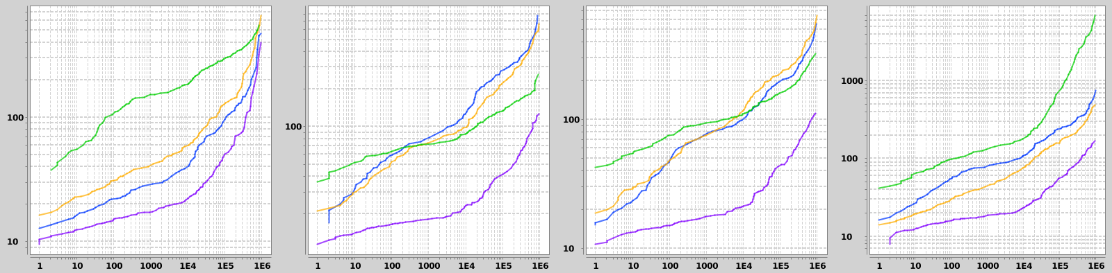
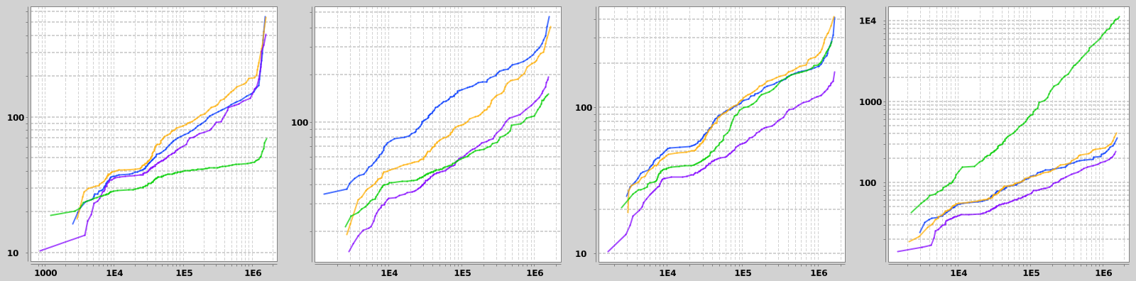
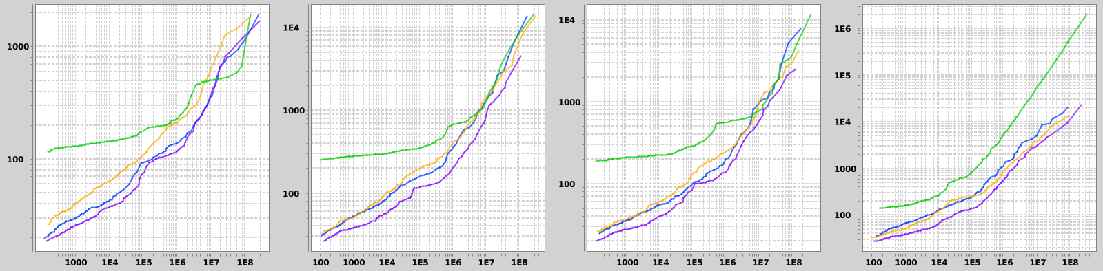
Re­sults from dif­fer­ent fil­ter-ag­gre­ga­tion com­bi­na­tions are shown in­fig­ures 1 - 3. Fil­ters are cho­sen at ran­dom at each run of the bench­mark, which means that num­ber of matches varies a lot. Thus I chose a bit un­ortho­dox method of vi­su­al­iz­ing the re­sults: x-axis is per­centiles (1 to 99) on the num­ber of match­ing rows and y-axis is per­centiles on query run­times. I did not check the rank cor­re­la­tion be­tween these val­ues but I ex­pect it to be rea­son­ably high. On all graphs the green line is the SQL Server with 32 GB of RAM, blue is Elas­tic­search with 16 GB, yel­low is ES with 32 GB and pur­ple is ES with 64 GB of RAM. In­ter­est­ingly dou­bling the mem­ory from 32 GB to 64 GB dropped query times by about 50% with Elas­tic­search. SQL Server per­formed best with sim­pler ag­gre­ga­tions, and per­formed rel­atively worst on the first fil­ter type (pre­sum­ably for not us­ing a spa­tial in­dex on lat/lon data) and the last ag­gre­ga­tion type, in which per­centiles were cal­cu­lated. At worst SQL Server was 10 - 40 times slower than Elas­tic­search.

Figure 1: Re­sults from the fil­ter tem­plate #1.

Figure 2: Re­sults from the fil­ter tem­plate #2.

Figure 3: Re­sults from the fil­ter tem­plate #3.

Related blog posts:

Analyzing NYC Taxi dataset with Elasticsearch and Kibana, 2017 Mar (Matching: Clojure, Databases, Elasticsearch, GitHub)
Very fuzzy searching with Elasticsearch, 2015 Oct (Matching: Databases, Elasticsearch, GitHub)
An efficient schema for hierarchical data on Elasticsearch, 2016 Nov (Matching: Databases, Elasticsearch)
Very fuzzy searching with CUDA, 2015 Nov (Matching: Databases, GitHub)
JGit blame for fun and profit(?), 2018 Apr (Matching: Clojure, Elasticsearch)