Niko's Project Corner

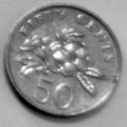
I de­vel­oped a coin recog­ni­tion sys­tem which can rec­og­nize eight dif­fer­ent groups of coins. The used set is all five coins of Sin­ga­pore, but a few cat­egories can­not be dis­tin­guished from each other with­out knowl­edge of the coin's size in re­la­tion to oth­ers.

I had ear­lier done a coin recog­ni­tion sys­tem, but it had only four cat­egories (10 and 20 cent Sin­ga­porean coins on both sides). The used pho­tos were de­lib­er­ately cor­rupted by very heavy JPG com­pres­sion, but I still felt the prob­lem wasn't fully solved. It used Sup­port Vec­tor Ma­chi­nes as the fi­nal clas­si­fier, and reached about 99% ac­cu­racy lev­els.

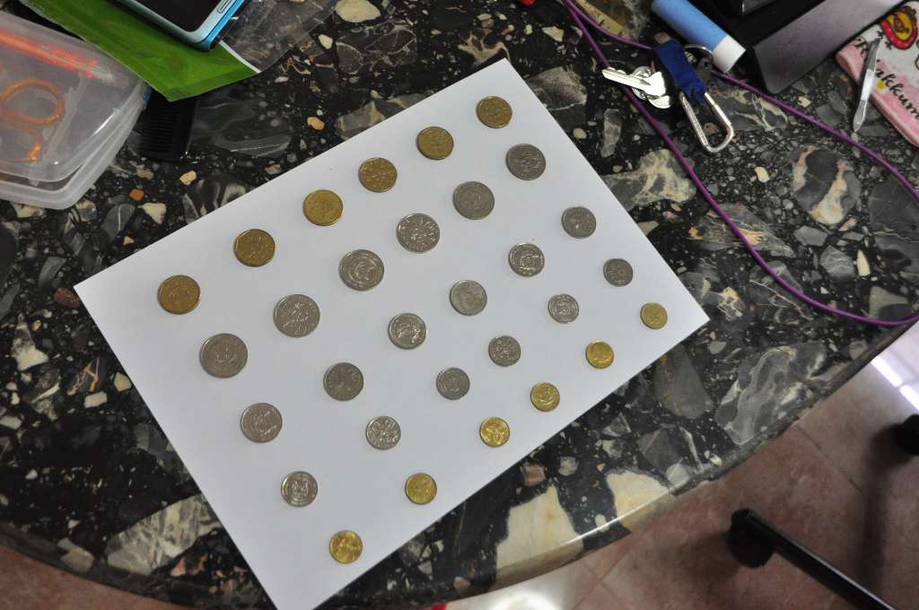
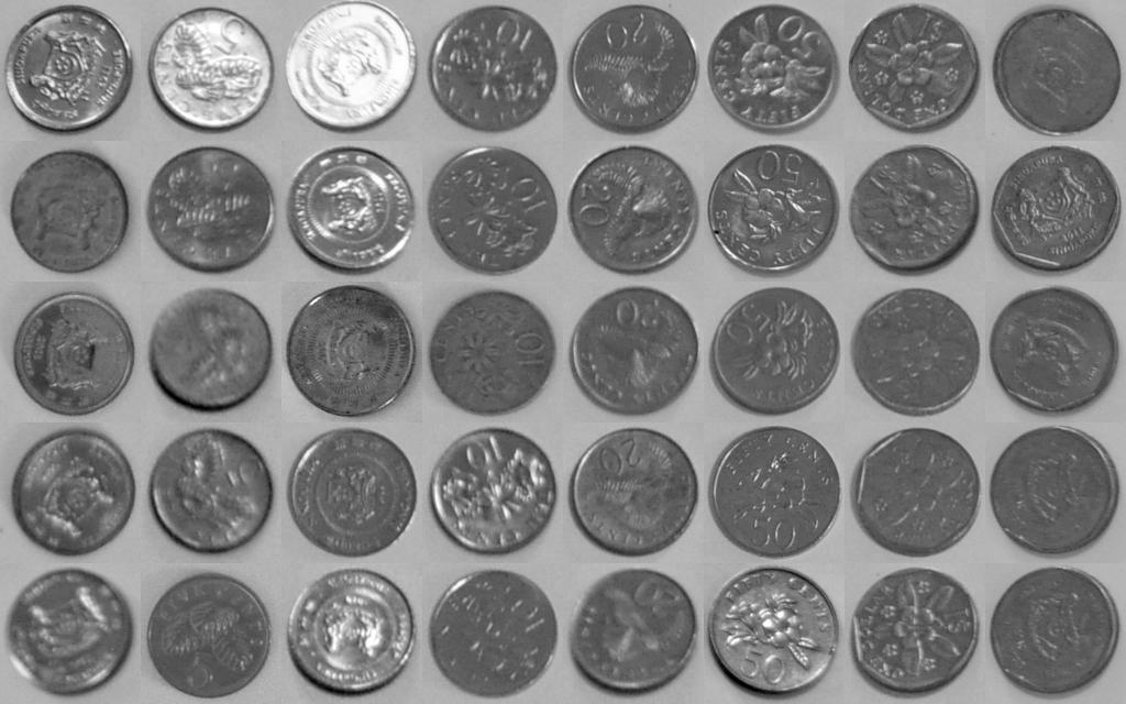
For the sec­ond round of ex­per­iments, I ar­ranged coins into a reg­ular pat­tern on a sheet of pa­per and took 40 pho­tos from dif­fer­ent an­gles. An ex­am­ple photo can be seen in Fig­ure 1. Coins were au­to­mat­ically ex­tracted from these im­ages, con­verted to grayscale, re­sized to 256 × 256 res­olu­tion and stored to a ded­icated folder. Then 30 ex­am­ple coins of each cat­egory were hand-picked and put to la­beled fold­ers, which were used as train­ing data for the su­per­vised learn­ing al­go­rithm. At this stage I re­al­ized that 10 cent and 50 cent coins had iden­ti­cal pat­tern, and also 5 cent and 20 cent coins.

Figure 1: An ex­am­ple photo of the coin im­age gath­er­ing.

The fea­ture ex­trac­tion pro­cess is shown in Fig­ure 2. It uti­lizes log-po­lar co­or­di­nates and the ab­so­lute value of Dis­crete Fourier Trans­form (DFT) to pro­duce ro­ta­tion and scale in­vari­ant de­scrip­tors. The cur­rent coin ex­trac­tion method is a bit in­ac­cu­rate in defin­ing the coin bound­aries, and thus the coin might not be cen­tered prop­erly in the cropped im­age. To make the sys­tem ro­bust against such er­rors, each coin in the train­ing set was dis­placed sev­eral times and these were treated as in­de­pen­dent train­ing ex­am­ples.

Figure 2: The fea­ture ex­trac­tion pro­cess: Orig­inal, lu­mi­nos­ity com­pen­sa­tion, log-po­lar co­or­di­nate trans­form and 1D DFT along the an­gu­lar com­po­nent.

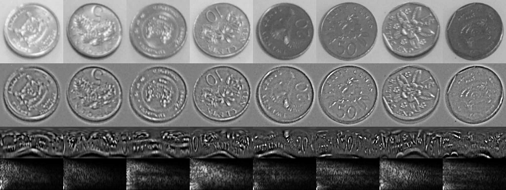
The used ma­chine learn­ing al­go­rithm is Lin­ear Dis­crim­inant Anal­ysis, be­cause it is easy to im­ple­ment and doesn't have many tun­ing pa­ram­eters. It also han­dles high-di­men­sional data with rel­ative ease, and in this case the data had 64 × 64 di­men­sions! This is the re­sult of first gen­er­at­ing 128 × 64 log-po­lar im­age, for which the DFT was cal­cu­lated. The ab­so­lute val­ues of this trans­form have re­dun­dancy in the data, and thus a 64 × 64 win­dow is suf­fi­cient. It is im­por­tant to note that the used DFT was done in 1D, not 2D as some­times is the case.

Figure 3: If the ro­ta­tion is cho­sen well, the data is al­most sep­ara­ble even in its two-di­men­sional pro­jec­tion. Pat­terns on the left rep­re­sent the lin­ear dis­crim­inant fea­tures.

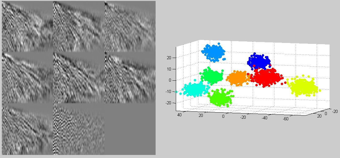
The Lin­ear Dis­crim­inant Anal­ysis was used to cre­ate 8 lin­ear clas­si­fiers (one for each class), each of which could dis­tin­guish items of the cor­re­spond­ing class from all other classes. This al­ready re­duces the dumber of di­men­sions from 4096 to 8, but ac­tu­ally that set of base vec­tors has only 7 de­grees of free­dom. The fi­nal post-pro­cess­ing step was to per­form Prin­ci­pal Com­po­nent Anal­ysis and drop the vec­tor with small­est eigen­value. This also helps with plot­ting the re­sult­ing point clouds, so that the within-class and be­tween-class co­vari­ance can be vi­su­ally ob­served. The re­sult­ing point clouds can be seen in Fig­ure 3. The odd look­ing pat­terns on the left are the lin­early dis­crim­inat­ing base vec­tors.

Once the data points have been trans­formed with the com­bined lin­ear trans­for­ma­tion of LDA and PCA, the data mean and co­vari­ances are cal­cu­lated. Dur­ing the match­ing stage these are used to cal­cu­late the Ma­ha­lanobis dis­tance from given point and each of the classes. Then met­rics such as the dis­tance from clos­est clus­ter, and the ra­tio of dis­tances to 1^st and 2^nd clos­est clus­ters can be used to de­ter­mine the most likely la­bel, and also es­ti­mate the like­li­hood of the es­ti­mate be­ing cor­rect.

Figure 4: A set of rec­og­nized coins, grouped in columns.

Ex­am­ples of cor­rectly iden­ti­fied coins can be seen in Fig­ure 4. Some of the coins are dif­fi­cult to rec­og­nize even for a per­son who is used to han­dle these coins, be­cause the high-con­trast de­tails might be lost. The sys­tem could be im­proved my com­pen­sat­ing for view point dif­fer­ences, which causes the coin to have an el­lipse-like shape.

In fu­ture I might add more train­ing data, la­belled test data and ROC (Re­ceiver Op­er­at­ing Char­ac­ter­is­tics) plots. Also in case some of the coins can be rec­og­nized, this gives us valu­able in­for­ma­tion about the rel­ative scale of the coins. This would en­able us to dis­tin­guish be­tween back sides of 10 and 50 cent coins, and solve other am­bigu­ous sit­ua­tions by us­ing be­lief prop­aga­tion meth­ods. I haven't use those in prac­tice yet, but they don't seem to be too com­pli­cated to im­ple­ment.

Related blog posts:

Cheating at Bananagrams with real-time AI, part 1, 2023 Apr (Matching: Computer Vision)
Introduction to Stable Diffusion's parameters, 2022 Nov (Matching: Computer Vision)
Matching puzzle pieces together, 2022 Jul (Matching: Computer Vision)
Single channel speech / music separation, 2022 Feb (Matching: FFT)
Image and video clustering with an autoencoder, 2022 Jan (Matching: Computer Vision)